Excel 2010's conditional formatting lets you change the appearance of a cell based on its value or another cell's value. You specify certain conditions, and when those conditions are met, Excel applies the formatting that you choose. You might use conditional formatting to locate dates that meet a certain criteria (such as falling on a Saturday or Sunday), to call out the highest or lowest values in a range, or to indicate values that fall under, over, or between specified amounts.
Select the cells to which you want to apply conditional formatting.
In most cases, you will select a single column or row of data in a table rather than an entire table.
On the Home tab, in the Styles group, click the Conditional Formatting button.
A menu appears with several different options for specifying the criteria.
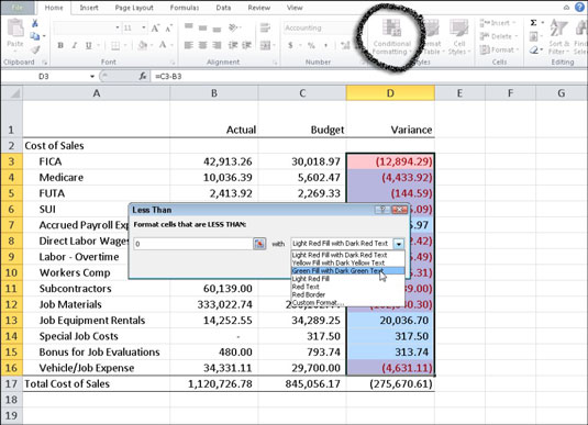
Point to Highlight Cells Rules and then select the type of criterion you want to use.

Criteria options include Greater Than, Less Than, Between, Equal To, Text That Contains, A Date Occurring, and Duplicate Values. A dialog box opens, where you can specify the values.
Enter the values you want to reference in the text box.
You can type a value here, such as 500, or you can reference a cell address, such as F12.
Click the drop-down arrow next to the format options and select the desired formatting.
Live Preview shows you what your data will look like. Click the Custom Format option if you want to create your own formatting selections.
Click OK.

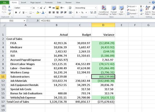
The cells that meet the specified criteria now appear with the chosen formatting options.


