When performing data analysis, you usually assume that your values cluster around some central data point (a median). But sometimes a few of the values fall too far from the central point. These values are called outliers (they lie outside the expected range). Outliers can skew your statistical analyses, leading you to false or misleading conclusions about your data.
You can use a few simple formulas and conditional formatting to highlight the outliers in your data.
The first step in identifying outliers is to pinpoint the statistical center of the range. To do this pinpointing, you start by finding the 1st and 3rd quartiles. A quartile is a statistical division of a data set into four equal groups, with each group making up 25 percent of the data. The top 25 percent of a collection is considered to be the 1st quartile, whereas the bottom 25 percent is considered the 4th quartile.
In Excel, you can easily get quartile values by using the QUARTILE function. This function requires two arguments: a range of data and the quartile number you want.
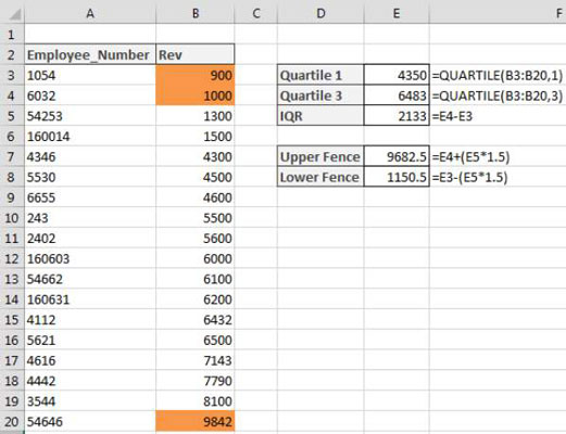
In the example shown, the values in cells E3 and E4 are the 1st and 3rd quartiles for the data in range B3:B20.

Taking these two quartiles, you can calculate the statistical 50 percent of the data set by subtracting the 3rd quartile from the 1st quartile. This statistical 50 percent is called the interquartile range (IQR). Figure 9-18 displays the IQR in cell E5.
Now the question is, how far from the middle 50 percent can a value sit and still be considered a “reasonable” value? Statisticians generally agree that IQR*1.5 can be used to establish a reasonable upper and lower fence:
The lower fence is equal to the 1st quartile – IQR*1.5.
The upper fence is equal to the 3rd quartile + IQR*1.5.
As you can see, cells E7 and E8 calculate the final upper and lower fences. Any value greater than the upper fence or less than the lower fence is considered an outlier.
At this point, the conditional formatting rule is easy to implement.
To build this basic formatting rule, follow these steps:
Select the data cells in your target range (cells B3:B20 in this example), click the Home tab of the Excel Ribbon, and then select Conditional Formatting→New Rule.
This opens the New Formatting Rule dialog box.

In the list box at the top of the dialog box, click the Use a Formula to Determine which Cells to Format option.
This selection evaluates values based on a formula that you specify. If a particular value evaluates to TRUE, the conditional formatting is applied to that cell.
In the formula input box, enter the formula shown here.
Note that you use the OR function to compare the value in your target cell (B3) to both the upper and lower fences found in cells $E$7 and $E$8, respectively. If the target cell is greater than the upper fence or less than the lower fence, it’s considered an outlier and thus will evaluate to TRUE, triggering the conditional formatting.
=OR(B3<$E$8,B3>$E$7)
Note that in the formula, you exclude the absolute reference dollar symbols ($) for the target cell (B3). If you click cell B3 instead of typing the cell reference, Excel automatically makes your cell reference absolute. It’s important that you don’t include the absolute reference dollar symbols in your target cell because you need Excel to apply this formatting rule based on each cell’s own value.
Click the Format button.
This opens the Format Cells dialog box, where you have a full set of options for formatting the font, border, and fill for your target cell. After you have completed choosing your formatting options, click the OK button to confirm your changes and return to the New Formatting Rule dialog box.
Back in the New Formatting Rule dialog box, click the OK button to confirm your formatting rule.
If you need to edit your conditional formatting rule, simply place your cursor in any of the data cells within your formatted range and then go to the Home tab and select Conditional Formatting→Manage Rules. This opens the Conditional Formatting Rules Manager dialog box. Click the rule that you want to edit then click the Edit Rule button.


