How to Find the Eigenfunctions of L2 in Spherical Coordinates

Your quantum physics instructor may ask you to find the eigenfunctions of L² in spherical coordinates. To do this, you start with the eigenfunction of

given that in spherical coordinates, the L² operator looks like this:

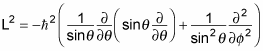
That’s quite an operator. And, given that

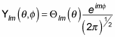
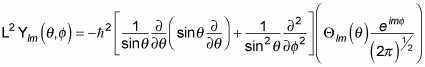
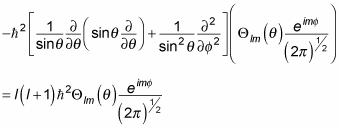
you can apply the L² operator to

which gives you the following:

And because

this equation becomes

Wow, what have you gotten into? Cancelling terms and subtracting the right-hand side from the left finally gives you this differential equation:

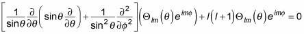
Combining terms and dividing by

gives you the following:

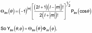
Holy cow! Isn’t there someone who’s tried to solve this kind of differential equation before? Yes, there is. This equation is a Legendre differential equation, and the solutions are well known. (Whew!) In general, the solutions take this form:

where

is the Legendre function.

So what are the Legendre functions? You can start by separating out the m dependence, which works this way with the Legendre functions:

where P_l(x) is called a Legendre polynomial and is given by the Rodrigues formula:

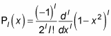
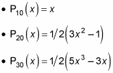
You can use this equation to derive the first few Legendre polynomials like this:

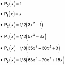
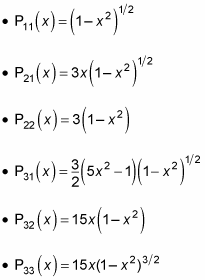
and so on. That’s what the first few P_l(x) polynomials look like. So what do the associated Legendre functions, P_lm(x) look like? You can also calculate them. You can start off with P_l0(x), where m = 0. Those are easy because P_l0(x) = P_l(x), so

Also, you can find that

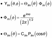
These equations give you an overview of what the P_lm functions look like, which means you’re almost done. As you may recall,

is related to the P_lm functions like this:

And now you know what the P_lm functions look like, but what do C_lm, the constants, look like? As soon as you have those, you’ll have the complete angular momentum eigenfunctions,

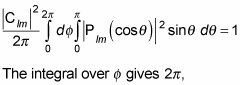
You can go about calculating the constants C_lm the way you always calculate such constants of integration in quantum physics — you normalize the eigenfunctions to 1.

that looks like this:

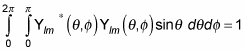
(Remember that the asterisk symbol [*] means the complex conjugate. A complex conjugate flips the sign connecting the real and imaginary parts of a complex number.)

Substitute the following three quantities in this equation:

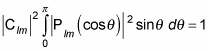
You get the following:

so this becomes

You can evaluate the integral to this:

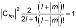
So in other words:

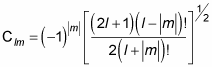
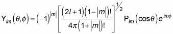
Which means that

which is the angular momentum eigenfunction in spherical coordinates, is

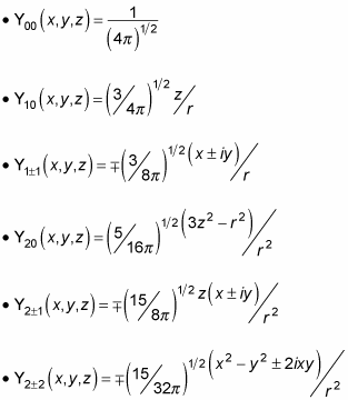
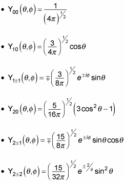
The functions given by this equation are called the normalized spherical harmonics. Here are what the first few normalized spherical harmonics look like:

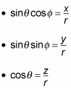
In fact, you can use these relations to convert the spherical harmonics to rectangular coordinates:

Substituting these equations into

gives you the spherical harmonics in rectangular coordinates: