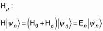
Using quantum physics, you can determine the f eigenvalues and matching eigenvectors for systems in which the energies are degenerate. Take a look at this unperturbed Hamiltonian:
![image0.png](https://www.dummies.com/wp-content/uploads/398142.image0.png)
In other words, several states have the same energy. Say the energy states are f-fold degenerate, like this:
![image1.png](https://www.dummies.com/wp-content/uploads/398143.image1.png)
How does this affect the perturbation picture? The complete Hamiltonian, H, is made up of the original, unperturbed Hamiltonian, H0, and the perturbation Hamiltonian,
![image2.png](https://www.dummies.com/wp-content/uploads/398144.image2.png)
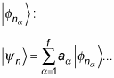
In zeroth-order approximation, you can write the eigenfunction
![image3.png](https://www.dummies.com/wp-content/uploads/398145.image3.png)
as a combination of the degenerate states
![image4.png](https://www.dummies.com/wp-content/uploads/398146.image4.png)
Note that in what follows, you assume that
![image5.png](https://www.dummies.com/wp-content/uploads/398147.image5.png)
if m is not equal to n. Also, you assume that the
![image6.png](https://www.dummies.com/wp-content/uploads/398148.image6.png)
are normalized — that is,
![image7.png](https://www.dummies.com/wp-content/uploads/398149.image7.png)
Plugging this zeroth-order equation into the complete Hamiltonian equation, you get
![image8.png](https://www.dummies.com/wp-content/uploads/398150.image8.png)
Now multiplying that equation by
![image9.png](https://www.dummies.com/wp-content/uploads/398151.image9.png)
gives you
![image10.png](https://www.dummies.com/wp-content/uploads/398152.image10.png)
Using the fact that
![image11.png](https://www.dummies.com/wp-content/uploads/398153.image11.png)
if m is not equal to n gives you
![image12.png](https://www.dummies.com/wp-content/uploads/398154.image12.png)
Physicists often write that equation as
![image13.png](https://www.dummies.com/wp-content/uploads/398155.image13.png)
where
![image14.png](https://www.dummies.com/wp-content/uploads/398156.image14.png)
And people also write that equation as
![image15.png](https://www.dummies.com/wp-content/uploads/398157.image15.png)
where E(1)n = En – E(0)n. That's a system of linear equations, and the solution exists only when the determinant to this array is nonvanishing:
![image16.png](https://www.dummies.com/wp-content/uploads/398158.image16.png)
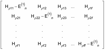
The determinant of this array is an fth degree equation in E(1)n, and it has f different roots,
![image17.png](https://www.dummies.com/wp-content/uploads/398159.image17.png)
Those f different roots are the first-order corrections to the Hamiltonian. Usually, those roots are different because of the applied perturbation. In other words, the perturbation typically gets rid of the degeneracy.
So here's the way you find the eigenvalues to the first order — you set up an f-by-f matrix of the perturbation Hamiltonian,
![image18.png](https://www.dummies.com/wp-content/uploads/398160.image18.png)
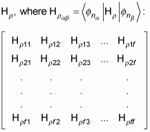
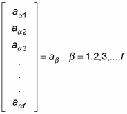
Then diagonalize this matrix and determine the f eigenvalues
![image19.png](https://www.dummies.com/wp-content/uploads/398161.image19.png)
and the matching eigenvectors:
![image20.png](https://www.dummies.com/wp-content/uploads/398162.image20.png)
Then you get the energy eigenvalues to first order this way:
![image21.png](https://www.dummies.com/wp-content/uploads/398163.image21.png)
And the eigenvectors are
![image22.png](https://www.dummies.com/wp-content/uploads/398164.image22.png)