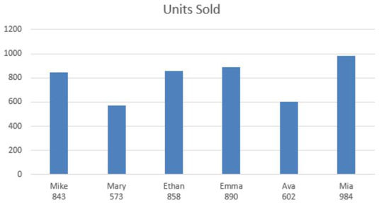
When creating charts in Excel, it’s sometimes useful to force line breaks for the purpose of composing better visualizations. Take the chart shown, for example. Here, the X-axis labels in the chart include the data value in addition to the sales rep. This setup works well when you don’t want to inundate your chart with data labels.

The secret to this trick is to use the CHAR() function in a formula that makes up your chart labels.

Every character in Excel has an associated ANSI character code. The ANSI character code is a Windows system code set that defines the characters you see on your screen. The ANSI character set consists of 255 characters, numbered from 1 to 255. The uppercase letter A is character number 97. The number 9 is character 57.
Even nonprinting characters have codes. The code for a space is 32. The code for a line break is 10.
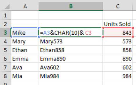
You can call up any character in a formula by using the CHAR() function. The example shown calls up the line break character and joins it with the values in cells A3 and C3:
=A3 & CHAR(10) & C3
The cell itself doesn’t show the line break unless you have wrap text applied. But even if you don’t, any chart using this kind of formula will display the data returned by the formula with the line breaks.


