One way to illustrate the binomial distribution is with a histogram. A histogram shows the possible values of a probability distribution as a series of vertical bars. The height of each bar reflects the probability of each value occurring. A histogram is a useful tool for visually analyzing the properties of a distribution, and (by the way) all discrete distributions may be represented with a histogram.
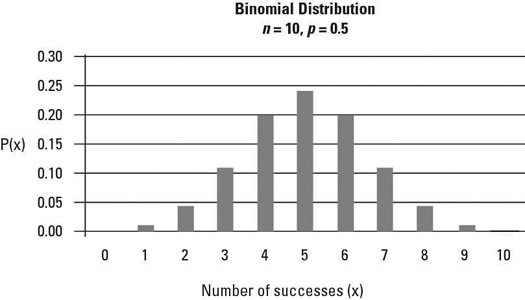
For example, suppose that a candy company produces both milk chocolate and dark chocolate candy bars. The product mix is 50 percent of the candy bars are milk chocolate and 50 percent are dark chocolate. Say you choose ten candy bars at random, and choosing milk chocolate is defined as a success. The probability distribution of the number of successes during these ten trials with p = 0.5 is shown here.

The figure shows that when p = 0.5, the distribution is symmetric about its expected value of 5 (np = 10[0.5] = 5), where the probabilities of X being below the mean match the probabilities of X being the same distance above the mean.
For example, with n = 10 and p = 0.5,
P(X = 4) = 0.2051 and P(X = 6) = 0.2051
P(X = 3) = 0.1172 and P(X = 7) = 0.1172
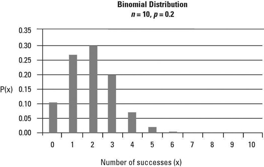
If the probability of success is less than 0.5, the distribution is positively skewed, meaning probabilities for X are greater for values below the expected value than above it.
For example, with n = 10 and p = 0.2,
P(X = 4) = 0.0881 and P(X = 6) = 0.0055
P(X = 3) = 0.2013 and P(X = 7) = 0.0008
This figure shows the probability distribution for n = 10 and p = 0.2.

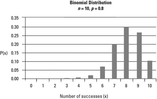
If the probability of success is greater than 0.5, the distribution is negatively skewed — probabilities for X are greater for values above the expected value than below it.
For example, with n = 10 and p = 0.8,
P(X = 4) = 0.0055 and P(X = 6) = 0.0881
P(X = 3) = 0.0008 and P(X = 7) = 0.2013
The final figure shows the probability distribution for the same situation when p = 0.8.


