The diffusion of new technology introduces a crucial time element into managerial decision-making. You may be interested in how an innovation is going to affect your firm’s production costs over time. Or you may be interested in determining how diffusion occurs within your firm’s industry. Learning curve and diffusion models examine the relationship between time and technological change and provide you perspective on how technological change evolves.
The learning curve for new technology
Adopting an innovation doesn’t necessarily result in an immediate reduction in production costs. Often on-the-job experience is necessary before you can take full advantage of the innovation. Learning-by-doing results in decreasing production cost per unit as the cumulative output produced increases, and firms use the innovation more efficiently. The relationship between cumulative output and production cost per unit is described by a learning curve.
It’s easy to mistakenly believe the new innovation’s adoption immediately leads to impressive gains in productivity and output. The day before the innovation, workers are using the old, inferior production method. The next day, the new production method leads to dramatic increases in productivity and lower production costs.
But many productivity gains are only realized after an extended period of time. With the passage of time, further improvements in production techniques occur as greater experience is gained. This accumulated learning leads to additional refinements in both production and organization that support additional productivity gains that further reduce production costs.
Given the learning curve, you may want to accept short-term losses in order to gain experience in producing a product. Setting a lower price encourages greater demand for the firm’s product, resulting in increased production. The learning-by-doing associated with the increased production results in lower per-unit cost on subsequent units produced, ultimately resulting in greater profits.
By accepting an initial loss through low prices and high production, you can take advantage of the learning curve in a shorter period of time, ultimately resulting in greater profits overall.
How to model diffusion to watch developments
The speed with which an innovation is adopted by firms in an industry is influenced by a number of factors. The most profitable innovations are adopted first. In addition, innovations requiring a small investment are typically adopted more readily than innovations requiring a substantial investment.
Iinnovations that have already been adopted by a large number of firms are more likely to be adopted by other firms due to increased information and competition.
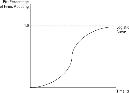
The relationship between diffusion, as measured by the percent of firms using an innovation, and time is often described by an S-shaped diffusion curve. Edwin Mansfield’s logistic curve often is used to describe this diffusion process. The formula for Mansfield’s logistic curve is

where P(t) represents the percentage of firms using the innovation at time t. The symbol e (Euler’s number) approximates to 2.718. The parameters α and β describe the diffusion process, and they vary among innovations. The function described by the logistic curve is illustrated below.

After you obtain data on the adoption of an innovation for previous years, you can estimate the logistic curve. After you estimate the curve, use it to predict the future diffusion path of the innovation. Firms have found that this technique has generated useful forecasts for the diffusion of a variety of innovations.


