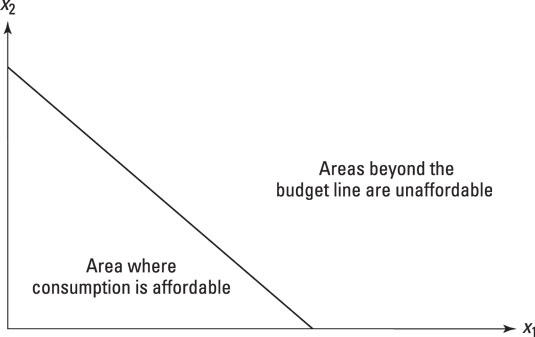
The key to moving from unconstrained optimization to constrained optimization is the introduction of a budget constraint. This is a method of conceptualizing all the ways that the choice of doing or buying something is held back by the availability of resources, whether in terms of money, time, or something else.
It also provides some insights that help economists put a bit more flesh on the utility model, bringing them closer to modeling the real world.
Imagine that you have two goods x1 and x2 — you can think of them as coffee and tea, or season tickets to see the Yankees and vacation days in Florida. Assume you have a fixed amount of resources, which you call M for now. The two goods have prices p1 and p2, respectively.
The maximum amount you can spend on both goods is M, and so the budget constraint has the following formula:
p1x1 + p2x2 = M
This equation is known as the budget line.
If you remember some of your high school algebra, you may have picked up that this equation describes a straight line, and that it slopes downward. By doing some rearranging in the equation, you can express the slope of the line by the price ratio of the two goods:
Slope = –p1 / p2
Any bundle of the goods x1 and x2 up to and including the budget line is feasible; anything beyond it is unfeasible and so is ruled out. The figure plots the shape of the set of feasible consumption choices.

Note that points or bundles beyond the budget line — that is, those farther away from the origin than the budget line — are now ruled out. This means that the highest possible indifference curve that you can be on is the one that is just touching or tangent in one place only to the budget constraint (assuming, that is, that the indifference curves are strictly convex).


