There will most definitely be times when you will need to work with the Z transformation in Six Sigma. How often do you come across a process or product characteristic that has an average of 0 and a standard deviation of 1? Not very often, if ever. So where’s the usefulness in the standard normal distribution and the standard normal probability tables?
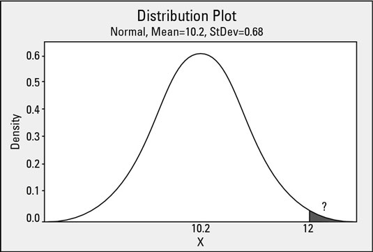
For example, what if a process characteristic you’re studying has an average of 10.2 and a standard deviation of 0.68, and you need to know what the probability is of observing a process value greater than 12.0? Why, you use the Z transformation, of course!

With this simple transformation of your process data, the standard normal distribution becomes highly useful. Consider the following mathematical transformation that changes your real-world data — which we call x — and scales them to the domain of the standard normal distribution:

What you’re doing mathematically is finding Z, the distance from your point of interest (x) to the real-world process average, and then calculating how many real-world standard deviations (s) you can fit within that distance. Try plugging in the values for the example situation:

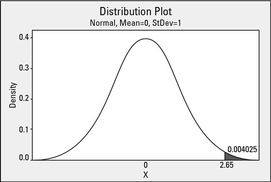
Figuring out the probability of observing a value greater than 12.0 on the curve is exactly the same as figuring out the probability of observing a value greater than 2.65 on the standard normal distribution.
Now that the problem is in the standard normal domain, you can use the standard normal probability table to find that the probability of being greater than 2.65 is 0.004025 (0.40 percent). This procedure holds for all situations where you are using a normal model to approximate your real-world data.


