


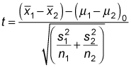
If the variances of two independent populations aren't equal (or you don't have any reason to believe that they're equal) and at least one sample is small (less than 30), the appropriate test statistic is
In this case, you get the critical values from the t-distribution with degrees of freedom (df) equal to
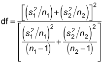
Note that this value isn't necessarily equal to a whole number; if the resulting value contains a fractional part, you must round it to the next closest whole number.
For example, assume that Major League Baseball (MLB) is interested in determining whether the mean number of runs scored per game is higher in the American League (AL) than in the National League (NL). The population variances are assumed to be unequal.
The first step is to assign one group to represent the first population ("population 1") and the other group to represent the second population ("population 2"). MLB designates the American League as population 1 and the National League as population 2.
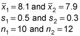
The next step is to choose samples from both populations. Suppose that MLB chooses a sample of 10 American League and 12 National League teams. The results are used to compute the sample mean and sample standard deviation for both leagues. Assume that the sample mean for runs scored among the AL games is 8.1, whereas the sample mean for the NL games is 7.9. The sample standard deviation is 0.5 for AL games and 0.3 for NL games.
MLB tests the null hypothesis that the population mean scores are equal at the 5 percent level of significance.
Here's a summary of the sample data:
The null hypothesis is
Because MLB is interested in determining whether the mean number of runs scored per game is higher in the American League than in the National League, you use a right-tailed test. The alternative hypothesis is
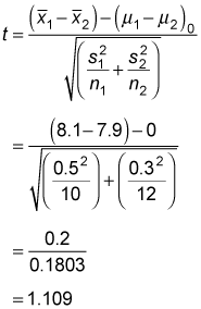
In other words, the test is designed to find strong evidence that the mean of population 1 is greater than the mean of population 2. You then solve the test statistic as follows:
And you find the degrees of freedom like so:
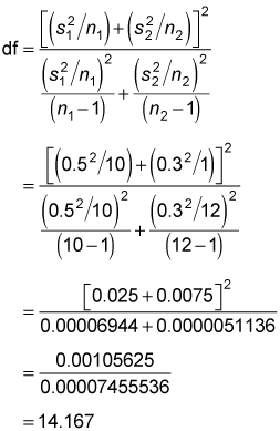
You round down the value of 14.167 to 14 because the degrees of freedom must be a whole number (or integer). With 14 degrees of freedom and a 5 percent level of significance, the critical value is
This result is obtained from the following table by finding the column headed t0.05 and the row corresponding to 14 degrees of freedom.
| Degrees of Freedom | t0.10 | t0.05 | t0.025 | t0.01 | t0.005 |
|---|---|---|---|---|---|
| 6 | 1.440 | 1.943 | 2.447 | 3.143 | 3.707 |
| 7 | 1.415 | 1.895 | 2.365 | 2.998 | 3.499 |
| 8 | 1.397 | 1.860 | 2.306 | 2.896 | 3.355 |
| 9 | 1.383 | 1.833 | 2.262 | 2.821 | 3.250 |
| 10 | 1.372 | 1.812 | 2.228 | 2.764 | 3.169 |
| 11 | 1.363 | 1.796 | 2.201 | 2.718 | 3.106 |
| 12 | 1.356 | 1.782 | 2.179 | 2.681 | 3.055 |
| 13 | 1.350 | 1.771 | 2.160 | 2.650 | 3.012 |
| 14 | 1.345 | 1.761 | 2.145 | 2.624 | 2.977 |
| 15 | 1.341 | 1.753 | 2.131 | 2.602 | 2.947 |
Because the test statistic (1.109) is below the critical value (1.761), the null hypothesis that
fails to be rejected. There's insufficient evidence to conclude that more runs are scored during American League games than National League games.


