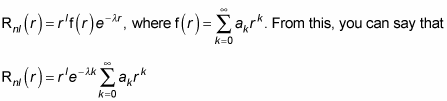
If your quantum physics instructor asks you to find the wave function of a hydrogen atom, you can start with the radial Schrödinger equation, Rnl(r), which tells you that
![image0.png](https://cdn.prod.website-files.com/6634a8f8dd9b2a63c9e6be83/669d4a5938584e222594bf45_396813.image0.png)
The preceding equation comes from solving the radial Schrödinger equation:
![image1.png](https://cdn.prod.website-files.com/6634a8f8dd9b2a63c9e6be83/669d4a5938584e222594bf42_396814.image1.png)
The solution is only good to a multiplicative constant, so you add such a constant, Anl (which turns out to depend on the principal quantum number n and the angular momentum quantum number l), like this:
![image2.png](https://cdn.prod.website-files.com/6634a8f8dd9b2a63c9e6be83/669d4a5938584e222594bf89_396815.image2.png)
You find Anl by normalizing Rnl(r).
Now try to solve for Rnl(r) by just flat-out doing the math. For example, try to find R10(r). In this case, n = 1 and l = 0. Then, because N + l + 1 = n, you have N = n – l – 1. So N = 0 here. That makes Rnl(r) look like this:
![image3.png](https://cdn.prod.website-files.com/6634a8f8dd9b2a63c9e6be83/669d4a5938584e222594bf4b_396816.image3.png)
And the summation in this equation is equal to
![image4.png](https://cdn.prod.website-files.com/6634a8f8dd9b2a63c9e6be83/669d4a5938584e222594bf5a_396817.image4.png)
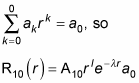
And because l = 0, rl = 1, so
![image5.png](https://cdn.prod.website-files.com/6634a8f8dd9b2a63c9e6be83/669d4a5938584e222594bf4f_396818.image5.png)
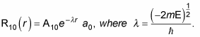
Therefore, you can also write
![image6.png](https://cdn.prod.website-files.com/6634a8f8dd9b2a63c9e6be83/669d4a5938584e222594bf7e_396819.image6.png)
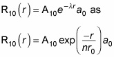
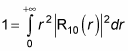
where r0 is the Bohr radius. To find A10 and a0, you normalize
![image7.png](https://cdn.prod.website-files.com/6634a8f8dd9b2a63c9e6be83/669d46b1ccb638857343e196_397915.image0.png)
to 1, which means integrating
![image8.png](https://cdn.prod.website-files.com/6634a8f8dd9b2a63c9e6be83/669d4a5938584e222594bf7b_396821.image8.png)
over all space and setting the result to 1.
![image9.png](https://cdn.prod.website-files.com/6634a8f8dd9b2a63c9e6be83/669d4a5938584e222594bf53_396822.image9.png)
and integrating the spherical harmonics, such as Y00, over a complete sphere,
![image10.png](https://cdn.prod.website-files.com/6634a8f8dd9b2a63c9e6be83/669d4a5938584e222594bf97_396823.image10.png)
gives you 1. Therefore, you’re left with the radial part to normalize:
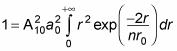
![image11.png](https://cdn.prod.website-files.com/6634a8f8dd9b2a63c9e6be83/669d4a5938584e222594bf61_396824.image11.png)
Plugging
![image12.png](https://cdn.prod.website-files.com/6634a8f8dd9b2a63c9e6be83/669d4a5938584e222594bf9e_396825.image12.png)
into
![image13.png](https://cdn.prod.website-files.com/6634a8f8dd9b2a63c9e6be83/669d4a5938584e222594bf61_396824.image11.png)
gives you
![image14.png](https://cdn.prod.website-files.com/6634a8f8dd9b2a63c9e6be83/669d4a5938584e222594bfa7_396827.image14.png)
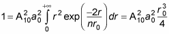
You can solve this kind of integral with the following relation:
![image15.png](https://cdn.prod.website-files.com/6634a8f8dd9b2a63c9e6be83/669d4a5938584e222594bf82_396828.image15.png)
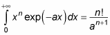
With this relation, the equation
![image16.png](https://cdn.prod.website-files.com/6634a8f8dd9b2a63c9e6be83/669d4a5938584e222594bf5d_396829.image16.png)
becomes
![image17.png](https://cdn.prod.website-files.com/6634a8f8dd9b2a63c9e6be83/669d4a5938584e222594bf78_396830.image17.png)
Therefore,
![image18.png](https://cdn.prod.website-files.com/6634a8f8dd9b2a63c9e6be83/669d4a5938584e222594bf85_396831.image18.png)
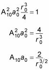
This is a fairly simple result. Because A10 is just there to normalize the result, you can set A10 to 1 (this wouldn’t be the case if
![image19.png](https://cdn.prod.website-files.com/6634a8f8dd9b2a63c9e6be83/669d4a5938584e222594bfaa_396832.image19.png)
involved multiple terms). Therefore,
![image20.png](https://cdn.prod.website-files.com/6634a8f8dd9b2a63c9e6be83/669d4a5938584e222594bf6a_396833.image20.png)
That’s fine, and it makes R10(r), which is
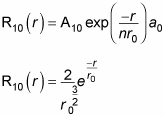
![image21.png](https://cdn.prod.website-files.com/6634a8f8dd9b2a63c9e6be83/669d4a5938584e222594bf6d_396834.image21.png)
You know that
![image22.png](https://cdn.prod.website-files.com/6634a8f8dd9b2a63c9e6be83/669d4a5938584e222594bfad_396835.image22.png)
And so
![image23.png](https://cdn.prod.website-files.com/6634a8f8dd9b2a63c9e6be83/669d46b1ccb638857343e196_397915.image0.png)
becomes
![image24.png](https://cdn.prod.website-files.com/6634a8f8dd9b2a63c9e6be83/669d4a5938584e222594bfa1_396837.image24.png)
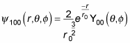
Whew. In general, here’s what the wave function
![image25.png](https://cdn.prod.website-files.com/6634a8f8dd9b2a63c9e6be83/669d46b00a1d7d1ef9d84941_397935.image3.png)
looks like for hydrogen:
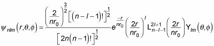
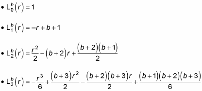
![image26.png](https://cdn.prod.website-files.com/6634a8f8dd9b2a63c9e6be83/669d4a5938584e222594bf94_396839.image26.png)
where
![image27.png](https://cdn.prod.website-files.com/6634a8f8dd9b2a63c9e6be83/669d4a5938584e222594bfa4_396840.image27.png)
is a generalized Laguerre polynomial. Here are the first few generalized Laguerre polynomials:
![image28.png](https://cdn.prod.website-files.com/6634a8f8dd9b2a63c9e6be83/669d4a5a38584e222594bfb7_396841.image28.png)