The most common financial functions in Excel 2010 — PV (Present Value) and FV (Future Value) — use the same arguments. The key to using these financial functions is to understand the terminology used by their arguments:
-
PV is the present value, the principal amount of the annuity.
-
FV is the future value, the principal plus interest on the annuity.
-
PMT is the payment made each period in the annuity. Normally, the payment is set over the life of the annuity and includes principal plus interest without any other fees.
-
RATE is the interest rate per period. Normally, the rate is expressed as an annual percentage.
-
NPER is the total number of payment periods in the life of the annuity. You calculate this number by taking the Term (the amount of time that interest is paid) and multiplying it by the Period (the point in time when interest is paid or earned) so that a loan with a three-year term with 12 monthly interest payments has 3 x 12, or 36 payment periods.
When using financial functions, keep in mind that the fv, pv, and pmt arguments can be positive or negative, depending on whether you're receiving the money or paying out the money. Also keep in mind that you want to express the rate argument in the same units as the nper argument, so that if you make monthly payments on a loan and you express the nper as the total number of monthly payments, as in 360 (30 x 12) for a 30-year mortgage, you need to express the annual interest rate in monthly terms as well.
Calculating the present value (PV)
The PV function returns the present value of an investment, which is the total amount that a series of future payments is worth presently. The syntax of the PV function is as follows:
=PV(rate,nper,pmt,[fv],[type])
The fv and type arguments are optional. The fv argument is the future value or cash balance that you want to have after making your last payment. If you omit the fv argument, Excel assumes a future value of zero. The type argument indicates whether the payment is made at the beginning or end of the period: Enter 0 (or omit the type argument) when the payment is made at the end of the period and use 1 when it is made at the beginning of the period.
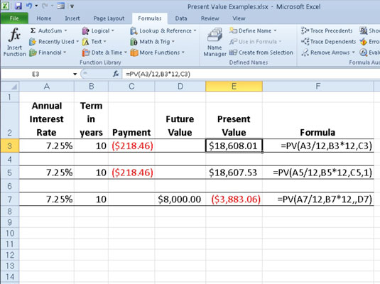
The following figure contains several examples using the PV function. All three PV functions use the same annual percentage rate of 7.25 percent and term of 10 years. Because payments are made monthly, each function converts these annual figures into monthly ones. For example, in the PV function in cell E3, the annual interest rate in cell A3 is converted into a monthly rate by dividing by 12 (A3/12) and the annual term in cell B3 is converted into equivalent monthly periods by multiplying by 12 (B3*12).

Determining the future value (FV)
The FV function calculates the future value of an investment. The syntax of this function is:
=FV(rate,nper,pmt,[pv],[type])
The rate, nper, pmt, and type arguments are the same as those used by the PV function. The pv argument is the present value or lump-sum amount for which you want to calculate the future value. As with the fv and type arguments in the PV function, both the pv and type arguments are optional in the FV function. If you omit these arguments, Excel assumes their values to be zero.
You can use the FV function to calculate the future value of an investment, such as an IRA (Individual Retirement Account). For example, suppose that you establish an IRA at age 43 and will retire 22 years hence at age 65 and that you plan to make annual payments into the IRA at the beginning of each year. If you assume a rate of return of 8.5 percent a year, you would enter the following FV function in your worksheet:
=FV(8.5%,22,-1000,,1)
Excel then indicates that you can expect a future value of $64,053.66 for your IRA when you retire at age 65. If you had established the IRA a year prior and the account already has a present value of $1,085, you would amend the FV function as follows:
=FV(8.5%,22,-1000,-1085,1)
In this case, Excel indicates that you can expect a future value of $70,583.22 for your IRA at retirement.


