


You can test different points to see which system is satisfied, often one at a time. Or you can look at a graph that gives you the overall view of the solutions.
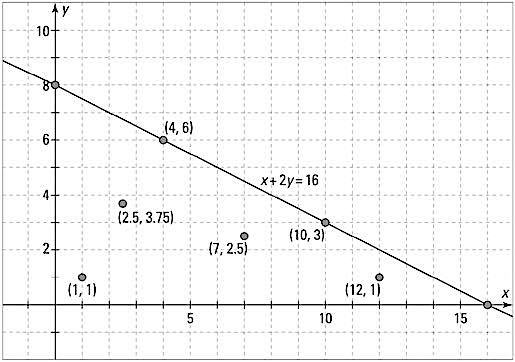
For example, you know that you can fit up to 16 ounces of a mixture of peanuts and almonds in your travel cup. An almond weighs twice as much as a peanut. So, what can you put in the cup? You can do 12 ounces of peanuts and 1 ounce of almonds, but there’s still room left. You can do 10 ounces of peanuts and 3 ounces of almonds. That should fit. Also, you can do 4 ounces of peanuts and 6 ounces of almonds, with room to spare. Many different combinations either fill the cup or leave room for more.
To examine this situation in a more orderly fashion, let x represent the number of ounces of peanuts and y represent the number of ounces of almonds. Remember that almonds weigh twice as much as peanuts.
The system of inequalities representing this situation is

The two inequalities, x ≥ 0 and y ≥ 0,
are what keep the graph of the system in the first quadrant. The values of x and y are never negative in a system with this requirement; they have to be positive or zero. In this almond-and-peanut situation, you can’t have a negative number of ounces, so the inequalities fit. This figure shows you the graph of the system.
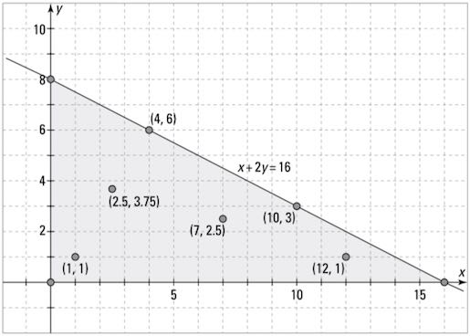
 All the points in the solution are in the triangular area.
You can’t possibly label all the points that fit the situation, so you just shade in the area that contains all the solutions. The next figure shows you the infinite number of choices. Of course, if you keep to sets of numbers lying on the line, you’ll have a full cup—the rest leave some room for more.
 Graph showing many ways to fill the cup.
Now, starting with a completely new situation working toward a system of inequalities, the graphs used in this new system show the graphs of the separate inequalities and then intersection of those inequalities. The graph of the system

consists of all the points in the intersection of the graphs of the two separate inequalities.
When graphing
![]()
if you use the test point (0, 0), you see that it doesn’t satisfy the inequality because
![]()
So, the shading is all above the line. When graphing
![]()
the test point (0, 0) does work because
![]()
so, you graph below the line to include the test point. The graph of
![]()
is shown here.

The graph of y ≤ x + 7 is shown here.

When both inequalities are graphed on the same coordinate axes, you can see what points they share. For example, in the next figure, you see that the points are all common solutions of the two inequalities. They are all solutions of the system.
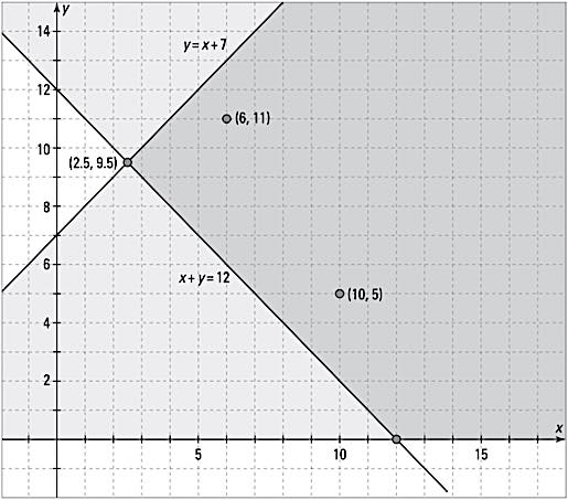 The two inequalities intersect and share points/solutions.

