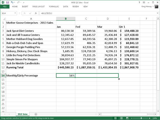
All new formulas you create in Excel 2013 naturally contain relative cell references unless you make them absolute. Because most copies you make of formulas require adjustments of their cell references, you rarely have to give this arrangement a second thought. Then, every once in a while, you come across an exception that calls for limiting when and how cell references are adjusted in copies.
One of the most common of these exceptions is when you want to compare a range of different values with a single value. This happens most often when you want to compute what percentage each part is to the total.
For example, in the Mother Goose Enterprises – 2013 Sales worksheet, you encounter this situation in creating and copying a formula that calculates what percentage each monthly total (in the cell range B14:D14) is of the quarterly total in cell E12.

Suppose that you want to enter these formulas in row 14 of the Mother Goose Enterprises – 2013 Sales worksheet, starting in cell B14. The formula in cell B14 for calculating the percentage of the January-sales-to-first-quarter-total is very straightforward:
=B12/E12
This formula divides the January sales total in cell B12 by the quarterly total in E12 (what could be easier?). Look, however, at what would happen if you dragged the fill handle one cell to the right to copy this formula to cell C14:
=C12/F12
The adjustment of the first cell reference from B12 to C12 is just what the doctor ordered. However, the adjustment of the second cell reference from E12 to F12 is a disaster. Not only do you not calculate what percentage the February sales in cell C12 are of the first quarter sales in E12, but you also end up with one of those horrible #DIV/0! error things in cell C14.
To stop Excel from adjusting a cell reference in a formula in any copies, convert the cell reference to absolute. To do this, press the function key F4, after you apply Edit mode (F2). You make the cell reference absolute by placing dollar signs in front of the column letter and row number. For example, cell B14 contains the correct formula to copy to the cell range C14:D14:
=B12/$E$12
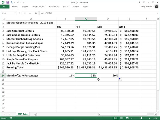
Look at the worksheet after this formula is copied to the range C14:D14 with the fill handle and cell C14 is selected. Notice that the Formula bar shows that this cell contains the following formula:

=C12/$E$12
Because E12 was changed to $E$12 in the original formula, all the copies have this same absolute (non-changing) reference.
If you goof up and copy a formula where one or more of the cell references should have been absolute but you left them all relative, edit the original formula as follows:
Double-click the cell with the formula or press F2 to edit it.
Position the insertion point somewhere on the reference you want to convert to absolute.
Press F4.
When you finish editing, click the Enter button on the Formula bar and then copy the formula to the messed-up cell range with the fill handle.
Be sure to press F4 only once to change a cell reference to completely absolute. If you press the F4 function key a second time, you end up with a so-called mixed reference, where only the row part is absolute and the column part is relative (as in E$12).
If you then press F4 again, Excel comes up with another type of mixed reference, where the column part is absolute and the row part is relative (as in $E12). If you press F4 yet again, Excel changes the cell reference back to completely relative (as in E12). After you’re back where you started, you can continue to use F4 to cycle through this same set of cell reference changes.
If you’re using Excel on a touchscreen device without access to a physical keyboard, the only way to convert cell addresses in your formulas from relative to absolute or some form of mixed address is to open the Touch keyboard and use it add the dollar signs before the column letter and/or row number in the appropriate cell address on the Formula bar.
Did this glimpse into Excel formulas leave you longing for more information and insight about Microsoft's popular spreadsheet program? You're free to test drive any of the For Dummies eLearning courses. Pick your course (you may be interested in more from Excel 2013), fill out a quick registration, and then give eLearning a spin with the Try It! button. You'll be right on course for more trusted know how: The full version's also available at Excel 2013.


