To the right of the Recommended Charts button in the Charts group of the Ribbon’s Insert tab in Excel 2013, you find particular command buttons with drop-down galleries for creating the following types and styles of charts:
![[Credit: ©iStockphoto.com/shironosov]](https://cdn.prod.website-files.com/6634a8f8dd9b2a63c9e6be83/6698cf5a097134be567cc05f_475344.image0.jpeg)
Insert Column Chart to preview your data as a 2-D or 3-D vertical column chart
Insert Bar Chart to preview your data as a 2-D or 3-D horizontal bar chart
Insert Stock, Surface or Radar Chart to preview your data as a 2-D stock chart (using typical stock symbols), 2-D or 3-D surface chart, or 3-D radar chart
Insert Line Chart to preview your data as a 2-D or 3-D line chart
Insert Area Chart to preview your data as a 2-D or 3-D area chart
Insert Combo Chart to preview your data as a 2-D combo clustered column and line chart or clustered column and stacked area chart
Insert Pie or Doughnut Chart to preview your data as a 2-D or 3-D pie chart or 2-D doughnut chart
Insert Scatter (X,Y) or Bubble Chart to preview your data as a 2-D scatter (X,Y) or bubble chart
When using the galleries attached to these chart command buttons on the Insert tab to preview your data as a particular chart style, you can embed the chart in your worksheet by simply clicking its chart icon.
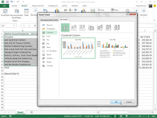
If you’re not sure what type of chart best represents your data, rather than go through the different chart type buttons on the Ribbon’s Insert tab, you can use the All Charts tab of the Insert Chart dialog box to try out your data in different chart types and styles.
You can open the Insert Chart dialog box by clicking the Dialog Box launcher in lower-right corner of the Charts group on the Insert tab and then display the complete list of chart types by clicking the All Charts tab in this dialog box.


