If you have a number of solutions to the Schrödinger equation, any linear combination of those solutions is also a solution. So that’s the key to getting a physical particle: You add various wave functions together so that you get a wave packet, which is a collection of wave functions of the form
![image0.png](https://cdn.prod.website-files.com/6634a8f8dd9b2a63c9e6be83/669d4a733494b70844ad9edb_396362.image0.png)
such that the wave functions interfere constructively at one location and interfere destructively (go to zero) at all other locations:
![image1.png](https://cdn.prod.website-files.com/6634a8f8dd9b2a63c9e6be83/669d4a733494b70844ad9edf_396363.image1.png)
This is usually written as a continuous integral:
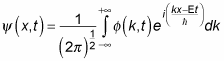
![image2.png](https://cdn.prod.website-files.com/6634a8f8dd9b2a63c9e6be83/669d4a733494b70844ad9efd_396364.image2.png)
What is
![image3.png](https://cdn.prod.website-files.com/6634a8f8dd9b2a63c9e6be83/669d4a733494b70844ad9f00_396365.image3.png)
It’s the amplitude of each component wave function, and you can find
![image4.png](https://cdn.prod.website-files.com/6634a8f8dd9b2a63c9e6be83/669d4a733494b70844ad9ed3_396366.image4.png)
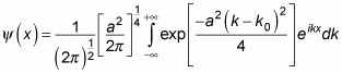
from the Fourier transform of the equation:
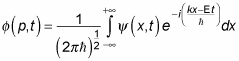
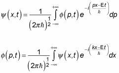
![image5.png](https://cdn.prod.website-files.com/6634a8f8dd9b2a63c9e6be83/669d4a733494b70844ad9ea8_396367.image5.png)
Because
![image6.png](https://cdn.prod.website-files.com/6634a8f8dd9b2a63c9e6be83/669d4a733494b70844ad9ee8_396368.image6.png)
you can also write the wave packet equations like this, in terms of p, not k:
![image7.png](https://cdn.prod.website-files.com/6634a8f8dd9b2a63c9e6be83/669d4a733494b70844ad9ed7_396369.image7.png)
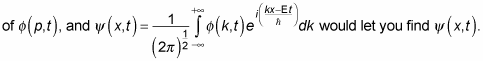
Well, you may be asking yourself just what’s going on here. It looks like
![image8.png](https://cdn.prod.website-files.com/6634a8f8dd9b2a63c9e6be83/669d4a733494b70844ad9ecd_396370.image8.png)
That looks pretty circular.
The answer is that the two previous equations aren’t definitions of
![image9.png](https://cdn.prod.website-files.com/6634a8f8dd9b2a63c9e6be83/669d4a733494b70844ad9ee5_396371.image9.png)
they’re just equations relating the two. You’re free to choose your own wave packet shape yourself — for example, you may specify the shape
![image10.png](https://cdn.prod.website-files.com/6634a8f8dd9b2a63c9e6be83/669d4a733494b70844ad9f1c_396372.image10.png)
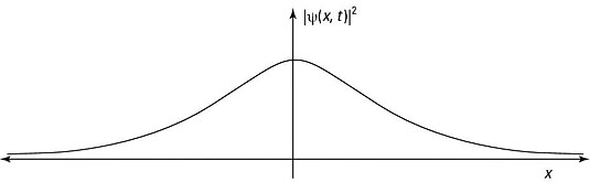
Here’s an example in which you get concrete, selecting an actual wave packet shape. Choose a so-called Gaussian wave packet, which you can see in the figure — localized in one place, close to zero in the others.
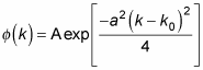
![A Gaussian wave packet.](https://cdn.prod.website-files.com/6634a8f8dd9b2a63c9e6be83/669d4a733494b70844ad9eeb_396373.image11.jpeg)
The amplitude
![image12.png](https://cdn.prod.website-files.com/6634a8f8dd9b2a63c9e6be83/669d4a733494b70844ad9ed0_396374.image12.png)
you may choose for this wave packet is
![image13.png](https://cdn.prod.website-files.com/6634a8f8dd9b2a63c9e6be83/669d4a733494b70844ad9efa_396375.image13.png)
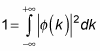
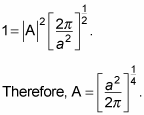
You start by normalizing
![image14.png](https://cdn.prod.website-files.com/6634a8f8dd9b2a63c9e6be83/669d4a733494b70844ad9ed0_396374.image12.png)
to determine what A is. Here’s how that works:
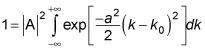
![image15.png](https://cdn.prod.website-files.com/6634a8f8dd9b2a63c9e6be83/669d4a733494b70844ad9f09_396377.image15.png)
Substituting in
![image16.png](https://cdn.prod.website-files.com/6634a8f8dd9b2a63c9e6be83/669d4a733494b70844ad9f06_396378.image16.png)
gives you this equation:
![image17.png](https://cdn.prod.website-files.com/6634a8f8dd9b2a63c9e6be83/669d4a733494b70844ad9f0c_396379.image17.png)
Doing the integral (that means looking it up in math tables) gives you the
following:
![image18.png](https://cdn.prod.website-files.com/6634a8f8dd9b2a63c9e6be83/669d4a733494b70844ad9f19_396380.image18.png)
So here’s your wave function:
![image19.png](https://cdn.prod.website-files.com/6634a8f8dd9b2a63c9e6be83/669d4a733494b70844ad9f12_396381.image19.png)
This little gem of an integral can be evaluated to give you the following:
![image20.png](https://cdn.prod.website-files.com/6634a8f8dd9b2a63c9e6be83/669d4a733494b70844ad9f0f_396382.image20.png)
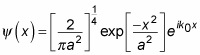
So that’s the wave function for this Gaussian wave packet (Note: The exp[–x2/a2] is the Gaussian part that gives the wave packet the distinctive shape that you see in the figure) — and it’s already normalized.
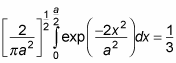
Now you can use this wave packet function to determine the probability that the particle will be in, say, the region
![image21.png](https://cdn.prod.website-files.com/6634a8f8dd9b2a63c9e6be83/669d4a733494b70844ad9f03_396383.image21.png)
The probability is
![image22.png](https://cdn.prod.website-files.com/6634a8f8dd9b2a63c9e6be83/669d4a733494b70844ad9ef4_396384.image22.png)
In this case, the integral is
![image23.png](https://cdn.prod.website-files.com/6634a8f8dd9b2a63c9e6be83/669d4a733494b70844ad9ef7_396385.image23.png)
And this works out to be
![image24.png](https://cdn.prod.website-files.com/6634a8f8dd9b2a63c9e6be83/669d4a733494b70844ad9ee2_396386.image24.png)
So the probability that the particle will be in the region
![image25.png](https://cdn.prod.website-files.com/6634a8f8dd9b2a63c9e6be83/669d4a733494b70844ad9f16_396387.image25.png)
Cool!