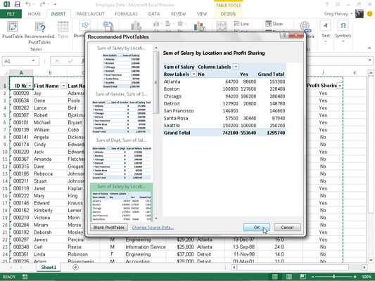
You can generate a new pivot table in Excel 2013 in a snap with the new Recommended Pivot Tables command button if creating a new pivot table with the Quick Analysis tool in Excel 2013 is too much work for you. To use this method, follow these easy steps:
Select a cell in the data list for which you want to create the new pivot table.
Provided that your data list has a row of column headings with contiguous rows of data, this can be any cell in the table.
Select the Recommended PivotTables command button on Insert tab of the Ribbon or press Alt+NSP.
Excel displays a Recommended PivotTables dialog box. This dialog box contains a list box on the left side that showing samples of all the suggested pivot tables that Excel 2013 can create from the data in your list.
Select the sample of the pivot table you want to create in the list box on the left and then click OK.
As soon as you click OK, Excel creates a new pivot table following the selected sample on its own worksheet (Sheet1) inserted in front of the others in your workbook. This pivot table is selected on the new sheet so that the Pivot Table Fields task pane is displayed on the right side of the Excel worksheet window and the PivotTable Tools contextual tab is displayed on the Ribbon.
You can use the options on this task pane and contextual tab to then customize your new pivot table.


