Add Excel Tables to the Power Pivot Data Model

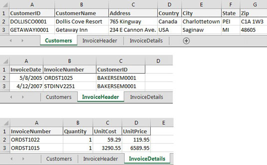
You want to use Power Pivot to analyze the data in the Customers, InvoiceHeader, and InvoiceDetails worksheets.

You can find the sample files for this exercise on in the workbook named Chapter 2 Samples.xlsx.

Follow these steps to add the newly created Excel tables to the data model using the Power Pivot tab:

1. Place the cursor anywhere inside the Customers Excel table.
2. Go to the Power Pivot tab on the Ribbon and click the Add to Data Model command.

The Power Pivot window shows all the data that exists in your data model.

Although the Power Pivot window looks like Excel, it's a separate program altogether. Notice that the grid for the Customers table has no row or column references. Also notice that you cannot edit the data within the table. This data is simply a snapshot of the Excel table you imported.

Additionally, if you look at the Windows taskbar at the bottom of the screen, you can see that Power Pivot has a separate window from Excel. You can switch between Excel and the Power Pivot window by clicking each respective program on the taskbar.

Repeat Steps 1 and 2 in the preceding list for your other Excel tables: Invoice Header, Invoice Details. After you've imported all your Excel tables into the data model, the Power Pivot window will show each dataset on its own tab, as shown.

Each table you add to the data model is placed on its own tab in Power Pivot.

The tabs in the Power Pivot window shown have a Hyperlink icon next to the tab names, indicating that the data contained in the tab is a linked Excel table. Even though the data is a snapshot of the data at the time you added it, the data automatically updates whenever you edit the source table in Excel.