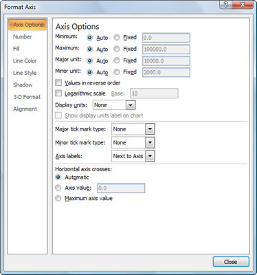
When charting values, Excel 2007 isn’t always careful how it formats the values that appear on the y-axis (or the x-axis when using some chart types, such as the 3-D Column chart or the XY Scatter chart).
If you’re not happy with the way the values appear on either the x-axis or y-axis, you can easily change the formatting.
Select the axis values you want to format.
Click the x-axis or y-axis directly in the chart or click the Chart Elements button (in the Current Selection group of the Format tab) and then click Horizontal (Category) Axis (for the x-axis) or Vertical (Value) Axis (for the y-axis) on its drop-down list. Be sure to select the axis values, not the axis title. Excel surrounds the axis you select with selection handles.
Click the Format Selection button in the Current Selection group of the Format tab.

Excel opens the Format Axis dialog box containing the following tabs: Axis Options, Number, Fill, Line Color, Line Style, Shadow, 3-D Format, and Alignment.
Change the appropriate options on the Axis Options tab as needed.
These options include those that fix the maximum and minimum amount for the first and last tick mark on the axis, display the values in reverse order (highest to lowest), apply a logarithmic scale, display units on the axis (hundreds, thousands, and millions, and so forth) and divide the values by those units, reposition the tick marks on the axis, and modify the value at which the other axis crosses.
Click the Number tab and change the number formatting as needed.
For example, to select the Number format with the comma as the thousands separator and no decimal places, you select Number in the Category list box; then leave the Use 1000 Separator (,) check box selected and enter 0 in the Decimal Places text box.
Click the Alignment tab and adjust how the labels appear.
Indicate the new orientation by clicking the desired vertical alignment in the Vertical Alignment drop-down list box and desired text direction in the Text Direction drop-down list.
Click Close.
As you choose new options for the selected axis, Excel 2007 shows you the change in the chart. These changes are, however, set in the chart only after you click Close in the Format Axis dialog box.
See also:
Customizing the Type and Style of an Excel 2007 Chart
Editing a Chart’s Date Source in Excel 2007


