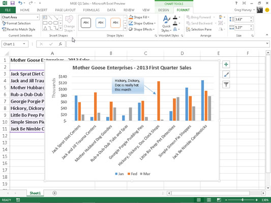
To add a text box in Excel 2013 like the one shown to the chart when a chart is selected, select the Format tab under the Chart Tools contextual tab. Then, click the Insert Shapes drop-down button to open its palette where you select the Text Box button.

To insert a text box in a worksheet when a chart or some other type of graphic isn’t selected, you can open the Insert tab on the Ribbon and then click the Text Box option on the Text button’s drop-down palette.
Excel then changes the mouse pointer or Touch Pointer to a narrow vertical line with a short cross near the bottom. Click the location where you want to draw the text box and then draw the box by dragging its outline. When you release the mouse button or remove your finger or stylus after dragging this pointer, Excel draws a text box in the shape and size of the outline.
After creating a horizontal text box, the program positions the insertion point at the top left, and you can then type the text you want to appear within it. The text you type appears in the text box and will wrap to a new line should you reach the right edge of the text box.
You can press Enter when you want to force text to appear on a new line. When you finish entering the message for your text box, click anywhere outside the box to deselect it.
After adding a text box to a chart or worksheet while it’s still selected, you can edit it as follows:
Move the text box to a new location in the chart by dragging it.
Resize the text box by dragging the appropriate sizing handle.
Rotate the text box by dragging its rotation handle (the green circle at the top) in a clockwise or counterclockwise direction.
Modify the formatting and appearance of the text box using the various command buttons in the Shape Styles group on the Format tab under the Drawing Tools contextual tab
Delete the text box by clicking its perimeter so that the dotted lines connecting the selection handles become solid and then pressing the Delete key.


