By assigning descriptive names to cell ranges, you can keep on top of the location of important information in an Excel 2016 worksheet. When assigning range names to a cell or cell range in Excel 2016, you need to follow a few guidelines:
Range names must begin with a letter of the alphabet, not a number.
For example, instead of 01Profit, use Profit01.
Range names cannot contain spaces.
Instead of a space, use the underscore (Shift+hyphen) to tie the parts of the name together. For example, instead of Profit 01, use Profit_01.
Range names cannot correspond to cell coordinates in the worksheet.
For example, you can't name a cell Q1 because this is a valid cell coordinate. Instead, use something like Q1_sales.
To name a cell or cell range in a worksheet, follow these steps:
Select the single cell or range of cells that you want to name.
Click the cell address for the current cell that appears in the Name Box on the far left of the Formula bar.
Excel selects the cell address in the Name Box.
Type the name for the selected cell or cell range in the Name Box.
When typing the range name, you must follow Excel's naming conventions: Refer to the bulleted list of cell-name do's and don'ts earlier in this section for details.
Press Enter.
To select a named cell or range in a worksheet, click the range name on the Name Box drop-down list. To open this list, click the drop-down arrow button that appears to the right of the cell address on the Formula bar.
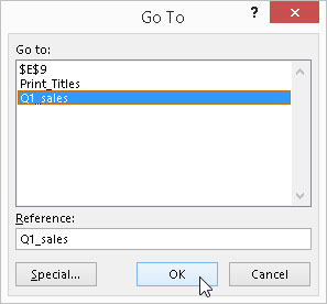
You can also accomplish the same thing by selecting Home→Find & Select (with the binoculars icon)→ Go To or by pressing F5 or Ctrl+G to open the Go To dialog box (see the figure). Double-click the desired range name in the Go To list box (alternatively, select the name followed by OK). Excel moves the cell cursor directly to the named cell. If you select a cell range, all the cells in that range are selected as well.


