Cell names are a great way to make out the purpose of your formulas in Excel 2013. For example, suppose that you have a simple formula in cell K3 that calculates the total due to you by multiplying the hours you work for a client (in cell I3) by the client’s hourly rate (in cell J3). Normally, you would enter this formula in cell K3 as
=I3*J3
However, if you assign the name Hours to cell I3 and the name Rate to cell J3, in cell K3 you could enter the formula
=Hours*Rate
The formula =Hours*Rate is much easier to understand than =I3*J3.
To enter a formula using cell names rather than cell references, follow these steps:
Assign range names to the individual cells.

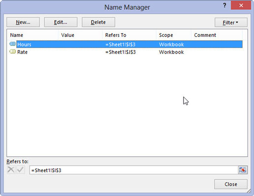
Click the Name Manager button in the Defined Names group on the Formulas tab of the ribbon. Give the name Hours to cell I3 and the name Rate to cell J3.
Create the formula.

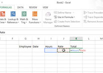
Put the cell cursor in cell K3. Type = (equal sign) to start the formula. Select the first cell referenced in the formula by selecting its cell (either by clicking the cell or moving the cell cursor into it). For this example, select the Hours cell by selecting cell I3.
Type the arithmetic operator to use in the formula. For this example, you would type * (asterisk) for multiplication.
Select the second cell referenced in the formula by selecting its cell (either by clicking the cell or moving the cell cursor into it). For this example, you select the Rate cell by selecting cell J3.
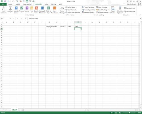
Click the Enter button or press Enter to complete the formula.

In this example, Excel enters the formula =Hours*Rate in cell K3.


