The AutoSum tool is in the Excel 2016 Editing group on the Home tab of the Ribbon. Look for the Greek sigma symbol. This little tool is worth its weight in gold when it comes to entering functions.
In addition to entering the SUM, AVERAGE, COUNT, MAX, or MIN functions, it also selects the most likely range of cells in the current column or row that you want to use as the function's argument and then automatically enters them as the function's argument.
Nine times out of ten, Excel selects (with the marquee or moving dotted line) the correct cell range to total, average, count, and so forth. For that tenth case, you can manually correct the range by simply dragging the cell pointer through the block of cells to sum.
Simply select the AutoSum button followed by Sum on the drop-down menu on the Home tab when you want to insert the SUM function into the current cell. The quicker method to select this function is to press Alt+= (the Alt key plus the equal to symbol on the top row).
If you want to use the AutoSum button to insert another function, such as AVERAGE, COUNT, MAX, or MIN, you need to click its drop-down button and select the name of the desired function on its pop-up menu (click Count Numbers on the menu to insert the COUNT function). If you select the More Functions command on this menu, Excel opens the Insert Function dialog box as though you had clicked the fx button on the Formula bar.
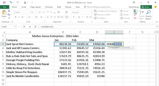
In the following figure, check out how to use AutoSum to total the sales of Jack Sprat Diet Centers in row 3. Position the cell pointer in cell E3 where the first-quarter total is to appear and then select Sum on the AutoSum drop-down menu (or press Alt+=). Excel inserts SUM (equal sign and all) onto the Formula bar; places a marquee around cells B3, C3, and D3; and uses the cell range B3:D3 as the argument of the SUM function.

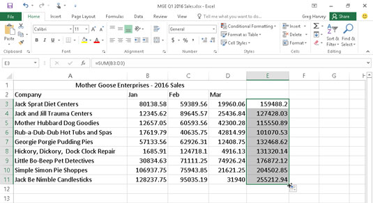
Now look at the worksheet after you insert the function in cell E3 (see the following figure). The calculated total appears in cell E3 while the following SUM function formula appears in the Formula bar:

=SUM(B3:D3)
After entering the function to total the sales of Jack Sprat Diet Centers, you can copy this formula to total sales for the rest of the companies by dragging the fill handle down column E until the cell range E3:E11 is highlighted (as shown).
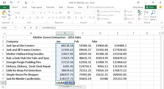
Look at the following figure to see how you can use AutoSum to total the January sales for all the Mother Goose Enterprises in column B. Position the cell pointer in cell B12 where you want the total to appear. Select Sum on the AutoSum's drop-down menu, and Excel places the marquee around cells B3 through B11 and correctly enters the cell range B3:B11 as the argument of the SUM function.

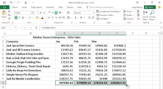
In the following figure, you see the worksheet after inserting the function in cell B12 and using the AutoFill feature to copy the formula to cells C12 and E12 to the right. (To use AutoFill, drag the fill handle through the cells to the right until you reach cell E12. Release the mouse button or remove your finger or stylus from the touchscreen.)


