


 You want to use Power Pivot to analyze the data in the Customers, InvoiceHeader, and InvoiceDetails worksheets.
You can find the sample files for this exercise on in the workbook named Chapter 2 Samples.xlsx.
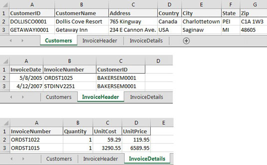
The Customers data set contains basic information, such as CustomerID, Customer Name, and Address. The InvoiceHeader data set contains data that points specific invoices to specific customers. The InvoiceDetails data set contains the specifics of each invoice.
To analyze revenue by customer and month, it's clear that you first need to somehow join these three tables together. In the past, you would have to go through a series of gyrations involving VLOOKUP or other clever formulas. But with Power Pivot, you can build these relationships in just a few clicks.
When linking Excel data to Power Pivot, best practice is to first convert the Excel data to explicitly named tables. Although not technically necessary, giving tables friendly names helps track and manage your data in the Power Pivot data model. If you don't convert your data to tables first, Excel does it for you and gives your tables useless names like Table1, Table2, and so on.
Follow these steps to convert each data set into an Excel table:
- Go to the Customers tab and click anywhere inside the data range.
- Press Ctrl+T on the keyboard.
This step opens the Create Table dialog box, shown here.
 Convert the data range into an Excel table.
 - In the Create Table dialog box, ensure that the range for the table is correct and that the My Table Has Headers check box is selected. Click the OK button. You should now see the Table Tools Design tab on the Ribbon.
- Click the Table Tools Design tab, and use the Table Name input to give your table a friendly name, as shown.
This step ensures that you can recognize the table when adding it to the Internal Data Model.
 Give your newly created Excel table a friendly name.
 - Repeat Steps 1 through 4 for the Invoice Header and Invoice Details data sets.

