For the PMP Certification Exam, you will need to know some terminology, measurements, and concepts in distribution. First, look at some definitions. Then, take a look at some basic statistics.
Probability distribution. A mathematical or graphical representation that represents the likelihood of different outcomes from a chance event.
Normal distribution. The frequently encountered bell-shaped distribution; the mean, median, and mode are the same value. Also known as a bell curve or a Gaussian distribution.
Cumulative distribution. A way to graph any distribution to show the probability that a given value and less (or more) will be achieved.
Mean. Also called the expected value, mean is the average of all data points. Mean may be computed as a simple average or a weighted average, based on a specific type of probability distribution, or by using a simulation.
Median. The point in the distribution where 50% of the results are above the value, and 50% of the results are below the value.
Mode. The most frequent data point.
Triangular distribution. A continuous distribution that is calculated by using three discrete variables or data points: optimistic, pessimistic, and most likely. They are not weighted in calculating the mean.
PERT distribution. A continuous distribution is calculated by using three discrete variables: optimistic, pessimistic, and most likely, of which most likely is weighted in calculating the mean.
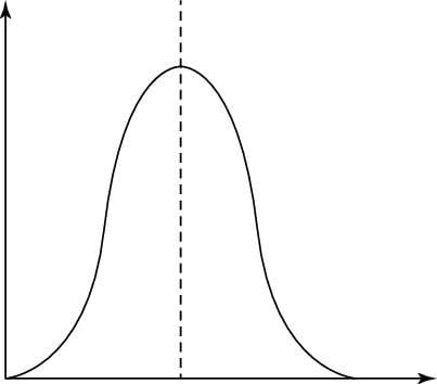
For the exam, all questions are based on a normal distribution. Here is a normal distribution curve.

In a normal distribution, the mean, median, and mode are all the same. That is the highest point of the curve. For a normal distribution, you’re looking at two aspects: the mean and the standard deviation. Standard deviation represents the distance a given point is from the mean. It is also called sigma, or s. Here is a more technical definition:
Standard deviation. A measure of the range of outcomes, the average difference from the mean, calculated as the square root of the variance. The symbol for standard deviation is σ.
The basic equation for computing standard deviation is

For the purposes of the PMP exam, you can use a shortcut. It works only for normal distributions, but because that’s all the PMP exam uses, you should be okay. The shortcut is
(pessimistic – optimistic) / 6
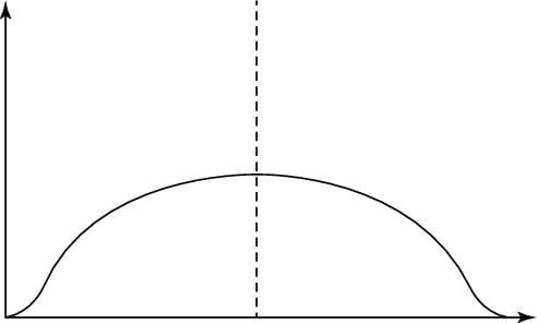
Basically, the mean shows the height of the curve, and the standard deviation determines the width of the curve. A narrow curve has a relatively low standard deviation. A flatter distribution has a relatively greater standard deviation.

Here is a wide distribution.

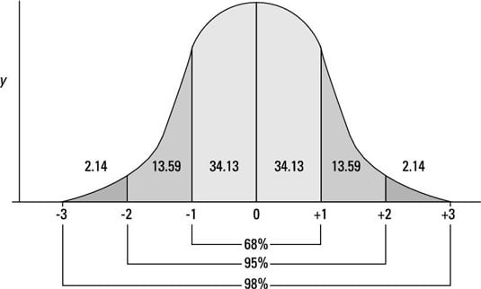
Generally, measurements are assessed by the number of standard deviations they are from the mean. In a normal distribution
68.3% of the data points fall within 1 standard deviation.
95.5% of the data points fall within 2 standard deviations.
99.7% of the data points fall within 3 standard deviations.
Thus, for a normal distribution, almost all values lie within 3 standard deviations of the mean.
You need this information for quality, cost-estimating, duration-estimation, and risk questions on the PMP exam. Here’s a quick example about project quality where you’re reviewing the quality of the duration estimates.
A team member estimates that Task A will most likely be finished in 30 days. The best case scenario is that it could be finished in 24 days, and the worst case scenario is that it would take 36 days. You would like estimates for expected completion. Based on this information, you want to know the answer to this question:
What is the probability that you will finish the task in 28–32 days?
To answer this question, take the following steps:
Calculate the mean (expected value) by using the PERT distribution equation.
(24 + 4(30) + 36) / 6 = 30
Calculate the standard deviation by using the short formula.
(36 – 24) / 6 = 2
Add and subtract the standard deviation value to and from the mean.
+/–1σis 28–32 days, which represents 68%.
So, you can reliably estimate a 68% chance that the activity will be finished within 28–32 days.
Here is one more piece of information you need to know: cumulative distribution. In a cumulative distribution, you will see the following:
0.15% of the data points fall between 0 and –3σfrom the mean.
2.25% of the data points fall between 0 and –2σfrom the mean.
16% of the data points fall between 0 and –1σfrom the mean.
84% of the data points fall between 0 and +1σfrom the mean.
97.75% of the data points fall between 0 and +2σfrom the mean.
99.85% of the data points fall between 0 and +3σfrom the mean.
Using the same question, calculate the probability of finishing in 32 days or less.
This question, though, is asking about the cumulative probability of all the values of 32 days or less. In Step 1 of the preceding list, the mean was 30 days. The standard deviation was 2. Take these steps to solve the problem:
30 days (the mean) +1ó(2 days) = 32 days.
Looking at the preceding information, you can see that 84% of the results fall between 0 and +1ófrom the mean.
Therefore, you can reliably estimate an 84% chance that the task will be finished in 32 days or less.
Because 68% of all results are +/–1σfrom the mean, if you are trying to determine the percent that is just +1σor just –1 σ, you divide 68% by 2 to get 34%. To get the cumulative distribution, you start with the mean of 50% and add 34% to show the cumulative value for +1 σ:
50% + (68% / 2) = 84%
You can subtract 34% to get the cumulative value for –1 σ:
50% – (68% / 2) = 16%
You follow the same method for 2σ using 95.5% divided by 2, and for 3σusing 99.7% divided by 2.

