All process and product data in Six Sigma projects have variation; each repeated instance of any measured data point is different from the instance before. And as the collection of repeated measurements piles up, a shape begins to form.
Real data usually cluster around a central value, and the occurrence of data points farther and farther from the central value tapers off. This setup is the classic bell-shaped kind of variation you constantly run across.
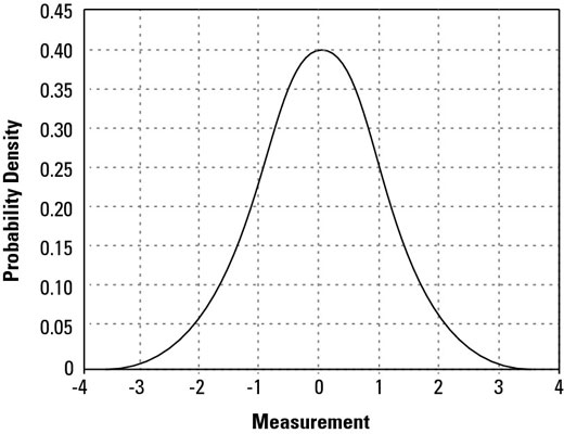
The normal model represents the density of all probabilities for a process or product characteristic — all past, current, and future occurrences of the characteristic in its present configuration.
The horizontal axis is scaled to units of the distribution’s standard deviation. And although the figure shows only the bell curve from –4 standard deviations to +4 standard deviations, it in fact extends out to negative infinity on the left and all the way to positive infinity on the right.
The vertical axis measures the probability density for each value of the measurement from negative infinity to positive infinity; the higher the bell curve, the greater the probability of the corresponding value on the horizontal axis occurring.
Notice that the normal curve is always positive; that is, its value is never zero or negative. It’s also perfectly symmetrical; if you fold the curve at its peak, the left and right halves match perfectly. The average value — called μ for the perfect model — occurs at the peak or center of the bell.
The standard deviation — called σ for the perfect model — is equivalent to the horizontal distance from the center of the curve (the average, or μ) to either point on the curve where its shape changes from concave to convex. In Figure 12-1, with the horizontal scale in units of standard deviations, you can see that this distance occurs at the measurement points of –1 and 1.
A final point to note about the normal model is that, if you measure the area enclosed by the bell curve and the horizontal axis, from negative infinity to positive infinity, it always equals 1. That is, the total area under the normal curve represents 100 percent of all possibilities — with 50 percent falling above the average and 50 percent below.
Working in from negative and positive infinity, if you calculate the area under the normal curve between –3 and +3 standard deviations, the result is 0.997, or 99.7 percent of the possible outcomes for the process characteristic. Farther in, between –2 and +2 standard deviations, about 95 percent all possibilities are captured. And 68 percent of all possibilities lie between –1 and +1 standard deviations.
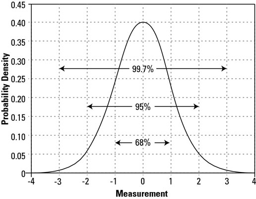
Because of the normal model’s symmetry, you can use these same area probabilities to determine the possibilities that lie beyond the parameters. For example, because 99.7 percent of all outcome possibilities lie between –3 and +3 standard deviations, you know that 0.3 percent of possibilities must lie beyond –3 and +3 standard deviations, with 0.15 percent lower than –3 standard deviations and 0.15 percent greater than +3 standard deviations.
And similarly, because about 95 percent of probabilities lie between –2 and +2 standard deviations, about 5 percent of probabilities must lie beyond –2 and +2 standard deviations. In all these examples, you can see that all the possibilities always combine to 100 percent.
Think about a special case of the normal model, where the average equals zero (μ = 0) and the standard deviation is equal to one (σ = 1). A normal distribution with these exact parameters is called the standard normal distribution.
Statisticians have spent a lot of time studying the standard normal distribution. One of the important things they have done is tabulate the area under the standard normal curve for various measurement values.
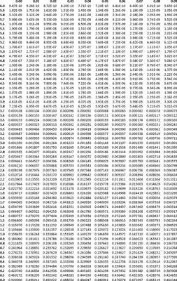
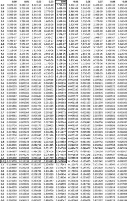
The row labels on the far left of this standard normal table correspond to various plus or minus distances from the zero center of the standard normal distribution. The column labels across the top row add a second decimal place to the distances. The cell contents correspond to the probability beyond the specified distance.
How to calculate the probability above or below a single value
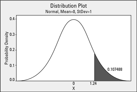
In the statistical tools of Six Sigma, you frequently calculate probabilities using the standard normal table. For example, you can easily look up the area under the standard normal curve greater than 1.24 in the table.
The probability from the table is 0.107488. So, for a normal distribution with mean of 0 and standard deviation of 1, the probability of observing a data value greater than 1.24 is 0.107488 (10.7 percent). Because of the symmetry of the model, this figure is also the exact probability of observing a value less than –1.24.
But that’s not all! Using the idea of complementary probabilities, you can calculate a 1 – 0.107488 = 0.892512 (89.3-percent) probability of observing a measurement less than 1.24 (and conversely, an 89.3-percent probability of observing a measurement greater than –1.24). Check out Figure 12-5 to see these probabilities in action.
How to calculate the probability between or outside two values
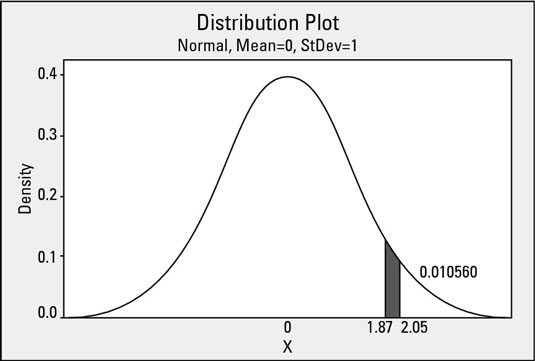
Figuring out probabilities with single values is relatively simple. Finding out how much area (probability) is under the standard normal curve between two finite values is only a little bit more difficult. For example, what is the area under the standard normal curve between the horizontal axis values of 1.87 and 2.05?
For that matter, how the heck are you supposed to determine that area if you can only look up one probability value in the standard normal probability table at a time?
On the flip side, you have a 1 – 0.10560 = 0.89440 (89.4 percent) probability of observing a value outside this interval. These probabilities correspond to a process characteristic that has an average of 0 and a standard deviation of 1.
