Statistical estimation theory focuses on the accuracy and precision of things that you estimate, measure, count, or calculate. It gives you ways to indicate how precise your measurements are and to calculate the range that's likely to include the true value.
Accuracy and precision
Whenever you estimate or measure anything, your estimated or measured value can differ from the truth in two ways — it can be inaccurate, imprecise, or both.
Accuracy refers to how close your measurement tends to come to the true value, without being systematically biased in one direction or another.
Precision refers to how close a bunch of replicate measurements come to each other — that is, how reproducible they are.
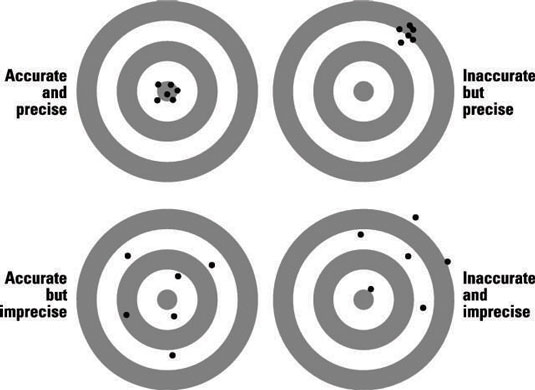
The figure shows four shooting targets with a bunch of bullet holes from repeated rifle shots. These targets illustrate the distinction between accuracy and precision — two terms that describe different kinds of errors that can occur when sampling or measuring something (or, in this case, when shooting at a target).

The upper-left target is what most people would hope to achieve — the shots all cluster together (good precision), and they center on the bull's-eye (good accuracy).
The upper-right target shows that the shots are all very consistent with each other (good precision), so we know that the shooter was very steady (with no large random perturbations from one shot to the next), and any other random effects must have also been quite small.
But the shots were all consistently high and to the right (poor accuracy). Perhaps the gun sight was misaligned or the shooter didn't know how to use it properly. A systematic error occurred somewhere in the aiming and shooting process.
The lower-left target indicates that the shooter wasn't very consistent from one shot to another (he had poor precision). Perhaps he was unsteady in holding the rifle; perhaps he breathed differently for each shot; perhaps the bullets were not all properly shaped, and had different aerodynamics; or any number of other random differences may have had an effect from one shot to the next.
About the only good thing you can say about this shooter is that at least he tended to be more or less centered around the bull's-eye — the shots don't show any tendency to be consistently high or low, or consistently to the left or right of center. There's no evidence of systematic error (or inaccuracy) in his shooting.
The lower-right target shows the worst kind of shooting — the shots are not closely clustered (poor precision) and they seem to show a tendency to be high and to the right (poor accuracy). Both random and systematic errors are prominent in this shooter's shooting.
Sampling distributions and standard errors
The standard error (abbreviated SE) is one way to indicate how precise your estimate or measurement of something is. The SE tells you how much the estimate or measured value might vary if you were to repeat the experiment or the measurement many times, using a different random sample from the same population each time and recording the value you obtained each time.
This collection of numbers would have a spread of values, forming what is called the sampling distribution for that variable. The SE is a measure of the width of the sampling distribution.
Fortunately, you don't have to repeat the entire experiment a large number of times to calculate the SE. You can usually estimate the SE using data from a single experiment.
Confidence intervals
Confidence intervals provide another way to indicate the precision of an estimate or measurement of something. A confidence interval (CI) around an estimated value is the range in which you have a certain degree of certitude, called the confidence level (CL), that the true value for that variable lies.
If calculated properly, your quoted confidence interval should encompass the true value a percentage of the time at least equal to the quoted confidence level.
Suppose you treat 100 randomly selected migraine headache sufferers with a new drug, and you find that 80 of them respond to the treatment (according to the response criteria you have established). Your observed response rate is 80 percent, but how precise is this observed rate?
You can calculate that the 95 percent confidence interval for this 80 percent response rate goes from 70.8 percent to 87.3 percent. Those two numbers are called the lower and upper 95 percent confidence limits around the observed response rate.
If you claim that the true response rate (in the population of migraine sufferers that you drew your sample from) lies between 70.8 percent and 87.3 percent, there's a 95 percent chance that that claim is correct.


