


A big wide world of properties is associated with signals and systems — plenty in the math alone! Here are ten unforgettable properties related to signals and systems work.
LTI system stability
Linear time-invariant (LTI) systems are bounded-input bounded-output (BIBO) stable if the region of convergence (ROC) in the s- and z-planes includes the
The s-plane applies to continuous-time systems, and the z-plane applies to discrete-time systems. But here’s the easy part: For causal systems, the property is poles in the left-half s-plane and poles inside the unit circle of the z-plane.
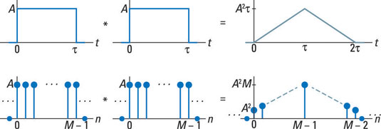
Convolving rectangles
The convolution of two identical rectangular-shaped pulses or sequences results in a triangle. The triangle peak is at the integral of the signal or sum of the sequence squared.
The convolution theorem
The four (linear) convolution theorems are Fourier transform (FT), discrete-time Fourier transform (DTFT), Laplace transform (LT), and z-transform (ZT).Note: The discrete-time Fourier transform (DFT) doesn’t count here because circular convolution is a bit different from the others in this set.
These four theorems have the same powerful result: Convolution in the time domain can be reduced to multiplication in the respective domains. For x1 and x2 signal or impulse response, y = x1 * x2becomes
Frequency response magnitude
For the continuous- and discrete-time domains, the frequency response magnitude of an LTI system is related to pole-zero geometry.
For continuous-time signals, you work in the s-domain; if the system is stable, you get the frequency response magnitude by evaluating |H(s)| along the jω-axis.
For discrete-time signals, you work in the z-domain; if the system is stable, you get the frequency response magnitude by evaluating |H(z)| around the unit circle as
In both cases, frequency response magnitude nulling occurs if either of the following values passes near or over a zero, and magnitude response peaking occurs if either of the following values passes near a pole:
The system can’t be stable if a pole is on either value.
Convolution with impulse functions
When you convolve anything with
you get that same anything back, but it’s shifted by t0 or n0. Case in point:

Spectrum at DC
The direct current (DC), or average value, of the signal x(t) impacts the corresponding frequency spectrum X(f) at f = 0. In the discrete-time domain, the same result holds for sequence x[n], except the periodicity of
in the discrete-time domain makes the DC component at
Frequency samples of N-point DFT
If you sample a continuous-time signal x(t) at rate fs samples per second to produce x[n] = x(n/fs), then you can load N samples of x[n] into a discrete-time Fourier transform (DFT) — or a fast Fourier transform (FFT), for which N is a power of 2. The DFT points k correspond to these continuous-time frequency values:
Assuming that x(t) is a real signal, the useful DFT points run from 0 to N/2.
Integrator and accumulator unstable
The integrator system Hi(s) = 1/s and accumulator system Hacc(z) = 1/(1 – z–1) are unstable by themselves. Why? A pole at s = 0 or a pole at z = 1 isn’t good. But you can use both systems to create a stable system by placing them in a feedback configuration. This figure shows stable systems built with the integrator and accumulator building blocks.

You can find the stable closed-loop system functions by doing the algebra:

The spectrum of a rectangular pulse
The spectrum of a rectangular pulse signal or sequence (which is the frequency response if you view the signal as the impulse response of a LTI system) has periodic spectral nulls. The relationship for continuous and discrete signals is shown here.

Odd half-wave symmetry and Fourier series harmonics
A periodic signal with odd half-wave symmetry,
is the period, has Fourier series representation consisting of only odd harmonics. If, for some constant A, y(t) = A + x(t), then the same property holds with the addition of a spectra line at f = 0 (DC). The square wave and triangle waveforms are both odd half-wave symmetric to within a constant offset.

