You can employ the least squares fit method in MATLAB. Least squares fit is a method of determining the best curve to fit a set of points. You can perform least squares fit with or without the Symbolic Math Toolbox.
Using MATLAB alone
In order to compute this information using just MATLAB, you need to do a lot of typing. The following steps get you started. The output is the parameters and the sum of the squares of the residuals. If you want to obtain additional information, such as the 95 percent confidence level used by some people, you need to perform additional coding.
Type XSource = 1:1:10; and press Enter.
Type YSource = [1, 2, 3.5, 5.5, 4, 3.9, 3.7, 2, 1.9, 1.5]; and press Enter.
The XSource and YSource vectors create a series of points to use for the least squares fit. The two vectors must be the same size.
Type plot(XSource, YSource) and press Enter.
You see a plot of the points which is helpful in visualizing how this process might work.

Type fun = @(p) sum((YSource - (p(1)*cos(p(2)*XSource)+p(2)*sin(p(1)*XSource))).^2); and press Enter.
This complex bit of typing is actually a function. You can use functions to automate the process of working with complex equations like this one. The equation is based on the least-squares-fitting methods described on various sites. The function accepts a single input — a guess as to the parameters for the least squares fit.
Type Guess = [2, 2]; and press Enter.
To make the function work, you have to provide a guess. Your guesses affect the output of the function, just as they do when performing the calculation manually.
Type [p, fminres] = fminsearch(fun, Guess) and press Enter.
The fminsearch() function accepts the function that you created and the guess that you made. Essentially, it performs unconstrained, nonlinear optimization of the function based on the guess that you provide. In this case, you see an output of
p =
 1.6204 1.8594
fminres =
 104.9327
When using this approach, you can use the output values of p for your next guess. In this case, you’d type Guess = [1.6204, 1.8594] and press Enter to change the guess value. Then you’d type [p, fminres] = fminsearch(fun, Guess) and press Enter to obtain the new output value of
p =
 1.6205 1.8594
fminres =
 104.9327
Using MATLAB with the Symbolic Math Toolbox
When working with the Symbolic Math Toolbox, you can use MuPAD to make things easier. In addition, the Symbolic Math Toolbox can greatly reduce the work you need to do by performing some of the calculations for you.
Open MuPAD by clicking the MuPAD Notebook entry on the Apps tab.
You see a new notebook open.
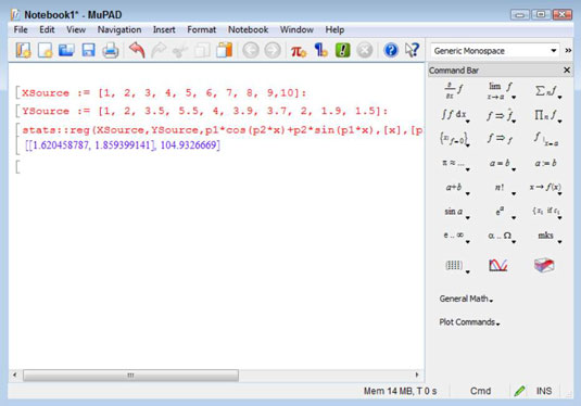
Type XSource := [1, 2, 3, 4, 5, 6, 7, 8, 9,10]: and press Enter.
This command creates the same XSource vector as that used for the previous example. To assign the vector to XSource, you use :=, rather than just the assignment operator used in MATLAB (=). Adding the colon (:) to the end of the statement keeps MuPAD from providing output.
Type YSource := [1, 2, 3.5, 5.5, 4, 3.9, 3.7, 2, 1.9, 1.5]: and press Enter.
You now have the points needed for the least squares fit.
Type stats::reg(XSource,YSource,p1*cos(p2*x)+p2*sin(p1*x),[x],[p1,p2],StartingValues=[2, 2]) and press Enter.
This long statement performs the same tasks as Steps 4, 5, and 6 in the preceding example. So, even though this example looks more complex, it actually saves steps.

The 1.620458778, 1859399122 part of the output are the parameters. You can use them to make your next guess.
Highlight the 2, 2 part of the equation and type 1.620458778, 1.859399122.
MuPAD replaces the old values with the new values you typed.
Press Enter.
You see the updated values. Again, they’re pretty close to the values output by the MATLAB-only solution.
Using the Symbolic Math Toolbox saves time and effort by reducing the number of steps you must take to find a solution. However, the output isn’t any different from working with MATLAB alone (a really good thing). The biggest time savings comes from being able to make guesses a lot faster and with greater ease.


