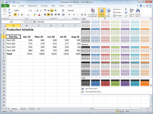
In Excel 2010, you can apply a predefined table format to a cell range. The Format as Table feature displays an extensive Table gallery with formatting thumbnails divided into three sections — Light, Medium, and Dark — each of which describes the intensity of the colors used by the various formats.
Click any cell within the group of cells you want to format as a table.
If you select multiple nonadjacent cells before you click the Format as Table button, the formats in the Table gallery are not available. This feature works with one contiguous group of cells.
On the Home tab, in the Styles group, click the Format as Table button.

A gallery of table formats appears. You can also build your own custom table format by clicking the New Table Style button below the table formats.
Click a thumbnail in the gallery.
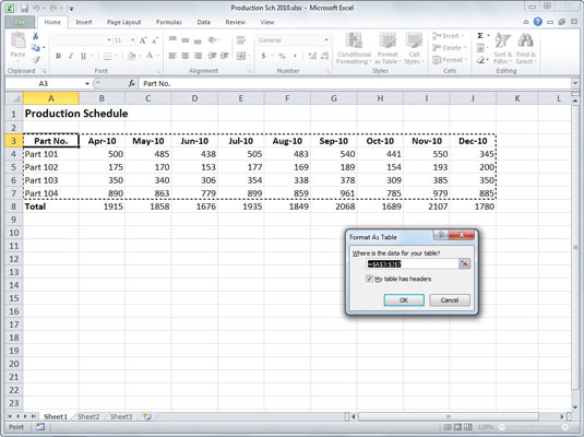
Excel makes its best guess as to the cell range of the table to apply it to (indicated by the marquee around its perimeter) and the Format As Table dialog box appears.
If the cell range for the table is incorrect, drag through the range in the worksheet.

The table range appears in the Where Is the Data for Your Table? text box.
Click OK.

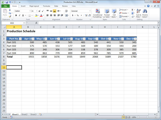
Excel formats the table with the style you selected, and the Table Tools Design contextual tab appears at the end of the Ribbon. Use the options on this tab to change the table style or modify other table settings.


