You can create a custom cell style from scratch in Excel 2013 by defining each of its formatting characteristics in the Style dialog box as follows:
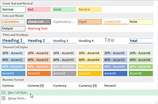
Position the cell pointer in a cell that doesn’t have any formatting applied to it and then click the New Cell Style option at the bottom of the Cell Styles drop-down gallery (opened by clicking the Cell Styles button in the Styles group on the Ribbon’s Home tab).
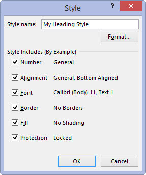
This action opens the Style dialog box with a generic style name (Style 1, Style 2, and so on), and with the attributes for the Normal style listed in the Style Includes (By Example) section of the dialog box.
Type a name for the new style that you are defining in the Style Name text box (replacing Style 1, Style 2, generic style name).
Now you need to select the formatting settings for the new style.
(Optional) Deselect the check box for any attribute (Number, Alignment, Font, Border, Fill, or Protection) that you don’t want included in the new style.
Click the Format button in the Style dialog box.
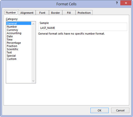
This action opens the standard Format Cells dialog box, where you can use the options on its six tabs (Number, Alignment, Font, Border, Fill, and Protection) to select all the formatting attributes that you do want used when you apply the new style to a cell selection.
After you finish assigning the formatting attributes that you want in the new style in the Format Cells dialog box, click OK to return to the Style dialog box.
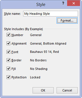
The Style Includes (By Example) section now lists all the attributes that you assigned in the Format Cells dialog box.
Click OK to close the Style dialog box.
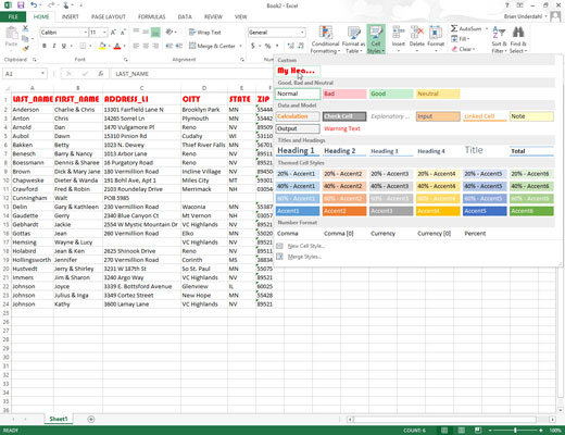
As soon as you click OK, Excel adds the new style to the Custom section of the Cell Styles gallery. To apply this new custom cell style to other cell selections in the worksheet, all you have to do is click its thumbnail in the Custom section of the gallery.


