How to Create an Excel 2019 Summary Report

Excel 2019 offers a ton of great features, including the summary report or summary worksheet. The Excel summary report recaps or totals the values stored in a bunch of other worksheets in the workbook.

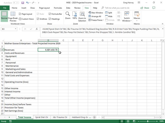
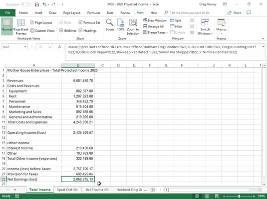
The best way that to learn how to create a summary worksheet is to walk through the procedure of making one (entitled Total Projected Income) for a fictional company. Let’s call it Mother Goose Enterprises – 2020 Projected Income workbook. This summary worksheet totals the projected revenue and expenses for all the companies that Mother Goose Enterprises operates.

Let’s assume the Mother Goose Enterprises – 2020 Projected Income workbook already contains nine worksheets with the 2020 projected revenue and expenses for each one of these companies, and that these worksheets are all laid out in the same arrangement. When you already have the necessary data entered into a workbook, creating this Excel summary report is a breeze:

1. Insert a new worksheet in front of the other worksheets in the MGE – 2020 Projected Income workbook and rename its sheet tab from Sheet1 to Total Income.
2. Next, enter the worksheet title Mother Goose Enterprises – Total Projected Income 2020 in cell A1.
   Do this by selecting cell A1 and then typing the text.

   Finally, copy the rest of the row headings for column A (containing the revenue and expense descriptions) from the Sprat Diet Ctr worksheet to the Total Income worksheet.

   To do this, select cell A3 in the Total Income sheet and then click the Sprat Diet Ctr tab. Select the cell range A3:A22 in this sheet; then press Ctrl+C, click the Total Income tab again, and press Enter.

You are now ready to create the master SUM formula that totals the revenues of all nine companies in cell B3 of the Total Income sheet:

1. Start by clicking cell B3 and pressing Alt+= to select the AutoSum feature.
   Excel then puts =SUM( ) in the cell with the insertion point placed between the two parentheses.
2. Click the Sprat Diet Ctr sheet tab, and then click its cell B3 to select the projected revenues for the Jack Sprat Diet Centers.
   The Formula bar reads =SUM('Sprat Diet Ctr'!B3) after selecting this cell.
3. Next, type a comma (,) — the comma starts a new argument. Click the J&J Trauma Ctr sheet tab and then click its cell B3 to select projected revenues for the Jack and Jill Trauma Centers.

   The Formula bar now reads =SUM('Sprat Diet Ctr'!B3,'J&J Trauma Ctr'!B3) after you select this cell.

4. Continue in this manner, typing a comma (to start a new argument) and then selecting cell B3 with the projected revenues for all the other companies in the following seven sheets.
   At the end of this procedure, the Formula bar now appears with the whopping SUM formula shown on the Formula bar.
5. To complete the SUM formula in cell B3 of the Total Income worksheet, click the Enter button in the Formula bar (You could press Enter on the keyboard, as well).
   Note the result in cell B3 below. As you can see in the Formula bar, the master SUM formula that returns 6,681,450.78 to cell B3 of the Total Income worksheet gets its result by summing the values in B3 in all nine of the supporting worksheets.

If you want to select the same cell across multiple worksheets, you can press and hold the Shift key, and then select the last worksheet. All worksheets in between the first and last will be included in the selection, or in this case, the calculation.

All that's left to do now is to use AutoFill to copy the master formula in cell B3 down to row 22, as follows:

1. With cell B3 still selected, drag the AutoFill handle in the lower-right corner of cell B3 down to cell B22 to copy the formula for summing the values for the nine companies down this column.
2. Then delete the SUM formulas from cells B4, B12, B14, B15, and B19 (all of which contain zeros because these cells have no income or expenses to total).

Here, you see the first section of the summary Total Income worksheet after you copy the formula created in cell B3 and after you delete the formulas from the cells that should be blank (all those that came up 0 in column B).