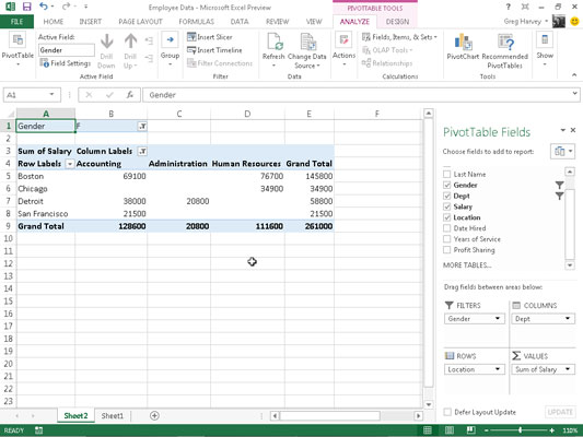
In Excel 2013, the filter buttons on the column and row fields attached to their labels enable you to filter out entries for particular groups and, in some cases, individual entries in the data source.
To filter the summary data in the columns or rows of a pivot table, click the column or row field’s filter button and click the check box at the top of the drop-down list to clear check marks. Click the check boxes for all the groups or entries whose summed values you want displayed in the pivot table to put back check marks in each box. Click OK.
As with filtering a Report Filter field, Excel replaces the standard drop-down button for that column or row field with a cone-shaped filter icon, indicating that the field is filtered and displaying only some of its summary values in the pivot table. To redisplay all the values for a filtered column or row field, click its filter button and then click at the top of its drop-down list. Click OK.
You can see the sample pivot table after filtering its Gender Report Filter field to women and its Dept Column field to Accounting, Administration, and Human Resources.

In addition to filtering out individual entries in a pivot table, you can also use the options on the Label Filters and Value Filters continuation menus to filter groups of entries that don’t meet certain criteria, such as company locations that don’t start with a particular letter or salaries between $45,000 and $65,000.


