You can use Excel’s Subtotals feature to subtotal data in a sorted list. To subtotal a data list, you first sort the list on the field for which you want the subtotals, and then you designate the field that contains the values you want summed — these don’t have to be the same fields in the data list.
When you use the Subtotals feature, you aren’t restricted to having the values in the designated field added together with the SUM function. You can instead have Excel return the number of entries with the COUNT function, the average of the entries with the AVERAGE function, the highest entry with the MAXIMUM function, the lowest entry with the MINIMUM function, or even the product of the entries with the PRODUCT function.
To subtotal the salaries within each department in my example Employee Data list, first sort the list in A-to-Z order on the Dept column because Excel is to create a new subtotal at each change in the department entries within the list (Accounting, Administration, Engineering, and so on).
Excel does not allow you to subtotal a data list formatted as a table. Before you can use the Subtotal command button, you must first convert your table into a normal range of cells. To do this, click a cell in the table and then click the Design tab on the Table Tools contextual tab on the Ribbon.
Finally, click the Convert to Range command button in the Tools group followed by the Yes button in the alert dialog box asking you to confirm this action. Excel then removes the filter buttons from the columns at the top of the data list while still retaining the original table formatting.
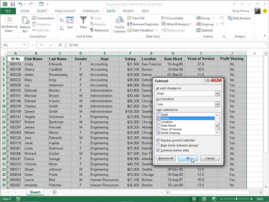
The following figure illustrates how easy it is to use the Subtotals feature to obtain totals in a data list. The sample Employee data list is sorted first by the Dept field in ascending order and then by the Salary field in descending order (Largest to Smallest) and converted the data list to a range.
Then click the Subtotal command button on the Ribbon’s Data tab to open the Subtotal dialog box.

Here, the Dept field is selected as the field for which the subtotals are to be calculated in the At Each Change In drop-down list box, Sum as the function to use in the Use Function drop-down list box, and the Salary check box as the field whose values are to be summed in the Add Subtotal To list box.
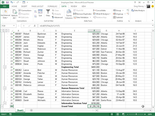
The following figure shows the results obtained after clicking OK in the Subtotal dialog box. Here, you see the bottom of the data list showing the salary subtotals for the Administration, Engineering, Human Resources, and Information Services departments along with the grand total of the salaries for all the departments.
The grand total is displayed at the bottom of the data list because the Summary below Data check box is selected in the Subtotal dialog box — if you didn't want a grand total, remove the check mark from this check box.

As you can see, when you use the Subtotals command, Excel outlines the data at the same time that it adds the rows with the departmental salary totals and the grand total. This means that you can collapse the data list down to just its departmental subtotal rows or even just the grand total row simply by collapsing the outline down to the second or first level.
(Remember that you can toggle between showing and hiding the outline symbols at the left edge of the data list by pressing Ctrl+8.)
In a large data list, you may want Excel to insert page breaks (often referred to as breaks) every time data changes in the field on which the list is being subtotaled (that is, the field designated in the At Each Change In drop-down list box).
To do this, you simply select the Page Break between Groups check box in the Subtotal dialog box to put a check mark in it before you click OK to subtotal the list.


