How Excel Formulas Work

Excel does lots of super cool things. In order to see them in all their glory, you need to understand how to work with Excel formulas. A formula, you may recall from the sleepy hours you spent in math class, is a way to calculate numbers. For example, 2+3=5 is a formula. When you enter a formula in a cell, Excel computes the formula and displays its results in the cell. Click in cell A3 and enter =2+3, for example, and Excel displays the number 5 in cell A3.

Referring to cells in formulas

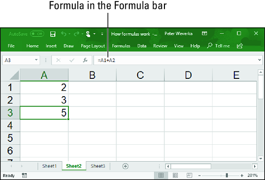
As well as numbers, Excel formulas can refer to the contents of different cells. When a formula refers to a cell, the number in the cell is used to compute the formula. In the image below, for example, cell A1 contains the number 2; cell A2 contains the number 3; and cell A3 contains the formula =A1+A2. As shown in cell A3, the result of the formula is 5. If you change the number in cell A1 from 2 to 3, the result of the formula in cell A3 (=A1+A2) becomes 6, not 5. When a formula refers to a cell and the number in the cell changes, the result of the formula changes as well.

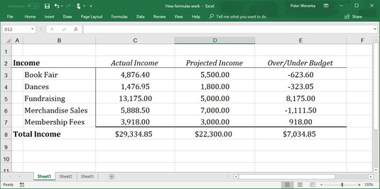
To see the value of using cell references in formulas, consider the worksheet shown below. The purpose of this worksheet is to track the budget of a school's Parent Teacher Association (PTA):

• Column C, Actual Income, lists income from different sources.
• Column D, Projected Income, shows what the PTA members thought income from these sources would be.
• Column E, Over/Under Budget, shows how actual income compares to projected income from the different sources.

As the figures in the Actual Income column (column C) are updated, figures in the Over/Under Budget column (column E) and the Total Income row (row 8) change instantaneously. These figures change instantaneously because the formulas refer to the numbers in cells, not to unchanging numbers (known as constants).

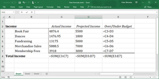
The image below shows the formulas used to calculate the data in the worksheet above. In column E, formulas deduct the numbers in column D from the numbers in column C to show where the PTA over- or under-budgeted for the different sources of income. In row 8, you can see how the SUM function is used to total cells in rows 3 through 7

Excel is remarkably good about updating cell references in formulas when you move cells. To see how good Excel is, consider what happens to cell addresses in formulas when you delete a row in a worksheet. If a formula refers to cell C1 but you delete row B, row C becomes row B and the value in cell C1 changes addresses from C1 to B1. You would think that references in formulas to cell C1 would be out of date, but you would be wrong. Excel automatically adjusts all formulas that refer to cell C1. Those formulas now refer to cell B1 instead.

In case you’re curious, you can display formulas in worksheet cells instead of the results of formulas by pressing Ctrl+’ (apostrophe) or clicking the Show Formulas button on the Formulas tab. (You may have to click the Formula Auditing button first, depending on the size of your screen.) Click the Show Formulas button a second time to see formula results again.

Referring to formula results in Excel 2019formulas

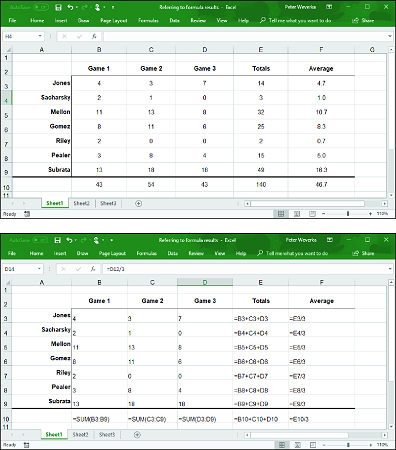
Besides referring to cells with numbers in them, you can refer to formula results in a cell. Consider the worksheet below. The purpose of this worksheet is to track scoring by the players on a basketball team over three games:

• The Totals column (column E) shows the total points each player scored in the three games.
• The Average column (column F), using the formula results in the Totals column, determines how much each player has scored on average. The Average column does that by dividing the results in column E by 3, the number of games played.

In this case, Excel uses the results of the total-calculation formulas in column E to compute average points per game in column F.

Operators in Excel 2019 formulas

Addition, subtraction, and division aren’t the only operators you can use in formulas. The table below explains the arithmetic operators you can use and the key you press to enter each operator. In the table, operators are listed in the order of precedence. Another way to compute a formula is to make use of a function. A function is a built-in formula that comes with Excel. SUM, for example, adds the numbers in cells. AVG finds the average of different numbers.

The order of precedence for Excel formulas

When a formula includes more than one operator, the order in which the operators appear in the formula matters a lot. Consider this formula:

=2+3*4

Does this formula result in 14 (2+[3*4>) or 20 ([2+3>*4)? The answer is 14 because Excel 2019 performs multiplication before addition in formulas. In other words, multiplication takes precedence over addition.

The order in which calculations are made in a formula that includes different operators is called the order of precedence. Be sure to remember the order of precedence when you construct complex formulas with more than one operator:

1. Percent (%)
2. Exponentiation (^)
3. Multiplication (*) and division (/); leftmost operations are calculated first
4. Addition (+) and subtraction (-); leftmost operations are calculated first
5. Concatenation (&)
6. Comparison (<, <=, >,>=, and <>)

To get around the order-of-precedence problem, enclose parts of formulas in parentheses. Operations in parentheses are calculated before all other parts of a formula. For example, the formula =2+3*4 equals 20 when it is written this way: =(2+3)*4.